Tutorial 7: ICE and PDP Interpretation Tutorial
![]()
Official LightAutoML github repository is here
Partial dependence plot (PDP) and Individual Conditional Expectation (ICE) are two model-agnostic interpretation methods (see details here).
Download library and make some imports
[1]:
# !pip install lightautoml
[2]:
# Standard python libraries
import os
import requests

# Installed libraries
import numpy as np
import matplotlib.pyplot as plt
import pandas as pd
import seaborn as sns
from sklearn.model_selection import train_test_split


# Imports from our package
from lightautoml.automl.presets.tabular_presets import TabularAutoML
from lightautoml.tasks import Task
[3]:
plt.rcParams.update({'font.size': 20})
sns.set(rc={'figure.figsize':(15, 11)})
sns.set(style="whitegrid", font_scale=1.5)

N_THREADS = 8 # threads cnt for lgbm and linear models
N_FOLDS = 5 # folds cnt for AutoML
RANDOM_STATE = 42 # fixed random state for various reasons
TEST_SIZE = 0.2 # Test size for metric check
TIMEOUT = 120 # Time in seconds for automl run
TARGET_NAME = 'TARGET' # Target column name
Prepare data
Load a dataset from the repository if doesn’t clone repository by git.
[4]:
DATASET_DIR = './data/'
DATASET_NAME = 'sampled_app_train.csv'
DATASET_FULLNAME = os.path.join(DATASET_DIR, DATASET_NAME)
DATASET_URL = 'https://raw.githubusercontent.com/AILab-MLTools/LightAutoML/master/examples/data/sampled_app_train.csv'
[5]:
%%time

if not os.path.exists(DATASET_FULLNAME):
    os.makedirs(DATASET_DIR, exist_ok=True)

    dataset = requests.get(DATASET_URL).text
    with open(DATASET_FULLNAME, 'w') as output:
        output.write(dataset)

data = pd.read_csv(DATASET_FULLNAME)
data['EMP_DATE'] = (np.datetime64('2018-01-01') + np.clip(data['DAYS_EMPLOYED'], None, 0).astype(np.dtype('timedelta64[D]'))
                    ).astype(str)
CPU times: user 223 ms, sys: 52.9 ms, total: 276 ms
Wall time: 503 ms
[6]:
train_data, test_data = train_test_split(data,
                                         test_size=TEST_SIZE,
                                         stratify=data[TARGET_NAME],
                                         random_state=RANDOM_STATE)
Create AutoML from preset
Also works with lightautoml.automl.presets.tabular_presets.TabularUtilizedAutoML.
[7]:
%%time

task = Task('binary', )
roles = {'target': TARGET_NAME,}

automl = TabularAutoML(task = task,
                       timeout = TIMEOUT,
                       cpu_limit = N_THREADS,
                       reader_params = {'n_jobs': N_THREADS, 'cv': N_FOLDS, 'random_state': RANDOM_STATE},
                      )
oof_pred = automl.fit_predict(train_data, roles = roles, verbose = 1, log_file = 'train.log')
[16:58:33] Stdout logging level is INFO.
[16:58:33] Copying TaskTimer may affect the parent PipelineTimer, so copy will create new unlimited TaskTimer
[16:58:33] Task: binary

[16:58:33] Start automl preset with listed constraints:
[16:58:33] - time: 120.00 seconds
[16:58:33] - CPU: 8 cores
[16:58:33] - memory: 16 GB

[16:58:33] Train data shape: (8000, 123)

[16:58:36] Layer 1 train process start. Time left 117.58 secs
[16:58:36] Start fitting Lvl_0_Pipe_0_Mod_0_LinearL2 ...
[16:58:40] Fitting Lvl_0_Pipe_0_Mod_0_LinearL2 finished. score = 0.7340989893230383
[16:58:40] Lvl_0_Pipe_0_Mod_0_LinearL2 fitting and predicting completed
[16:58:40] Time left 112.94 secs

[16:58:43] Selector_LightGBM fitting and predicting completed
[16:58:44] Start fitting Lvl_0_Pipe_1_Mod_0_LightGBM ...
[16:58:53] Time limit exceeded after calculating fold 3

[16:58:53] Fitting Lvl_0_Pipe_1_Mod_0_LightGBM finished. score = 0.7336652733096534
[16:58:53] Lvl_0_Pipe_1_Mod_0_LightGBM fitting and predicting completed
[16:58:53] Start hyperparameters optimization for Lvl_0_Pipe_1_Mod_1_Tuned_LightGBM ... Time budget is 1.00 secs
[16:59:03] Hyperparameters optimization for Lvl_0_Pipe_1_Mod_1_Tuned_LightGBM completed
[16:59:03] Start fitting Lvl_0_Pipe_1_Mod_1_Tuned_LightGBM ...
[16:59:16] Fitting Lvl_0_Pipe_1_Mod_1_Tuned_LightGBM finished. score = 0.7146425170595188
[16:59:16] Lvl_0_Pipe_1_Mod_1_Tuned_LightGBM fitting and predicting completed
[16:59:16] Start fitting Lvl_0_Pipe_1_Mod_2_CatBoost ...
[16:59:21] Fitting Lvl_0_Pipe_1_Mod_2_CatBoost finished. score = 0.7180592042951911
[16:59:21] Lvl_0_Pipe_1_Mod_2_CatBoost fitting and predicting completed
[16:59:21] Start hyperparameters optimization for Lvl_0_Pipe_1_Mod_3_Tuned_CatBoost ... Time budget is 29.20 secs
[16:59:51] Hyperparameters optimization for Lvl_0_Pipe_1_Mod_3_Tuned_CatBoost completed
[16:59:51] Start fitting Lvl_0_Pipe_1_Mod_3_Tuned_CatBoost ...
[16:59:58] Fitting Lvl_0_Pipe_1_Mod_3_Tuned_CatBoost finished. score = 0.7424781750625415
[16:59:58] Lvl_0_Pipe_1_Mod_3_Tuned_CatBoost fitting and predicting completed
[16:59:58] Time left 35.17 secs

[16:59:58] Time limit exceeded in one of the tasks. AutoML will blend level 1 models.

[16:59:58] Layer 1 training completed.

[16:59:58] Blending: optimization starts with equal weights and score 0.7470969001073415
[16:59:58] Blending: iteration 0: score = 0.7483672886691461, weights = [0.18754406 0.1279657  0.37286162 0.06386749 0.24776113]
[16:59:58] Blending: iteration 1: score = 0.7484541355819561, weights = [0.23439428 0.12674679 0.31599942 0.06325912 0.25960034]
[16:59:59] Blending: iteration 2: score = 0.748450627689517, weights = [0.23445104 0.1267374  0.315976   0.06325444 0.25958112]
[16:59:59] Blending: iteration 3: score = 0.748450627689517, weights = [0.23445104 0.1267374  0.315976   0.06325444 0.25958112]
[16:59:59] Blending: no score update. Terminated

[16:59:59] Automl preset training completed in 85.25 seconds

[16:59:59] Model description:
Final prediction for new objects (level 0) =
         0.23445 * (5 averaged models Lvl_0_Pipe_0_Mod_0_LinearL2) +
         0.12674 * (4 averaged models Lvl_0_Pipe_1_Mod_0_LightGBM) +
         0.31598 * (5 averaged models Lvl_0_Pipe_1_Mod_1_Tuned_LightGBM) +
         0.06325 * (5 averaged models Lvl_0_Pipe_1_Mod_2_CatBoost) +
         0.25958 * (5 averaged models Lvl_0_Pipe_1_Mod_3_Tuned_CatBoost)

CPU times: user 10min 7s, sys: 49.1 s, total: 10min 56s
Wall time: 1min 25s
Calculate interpretation data
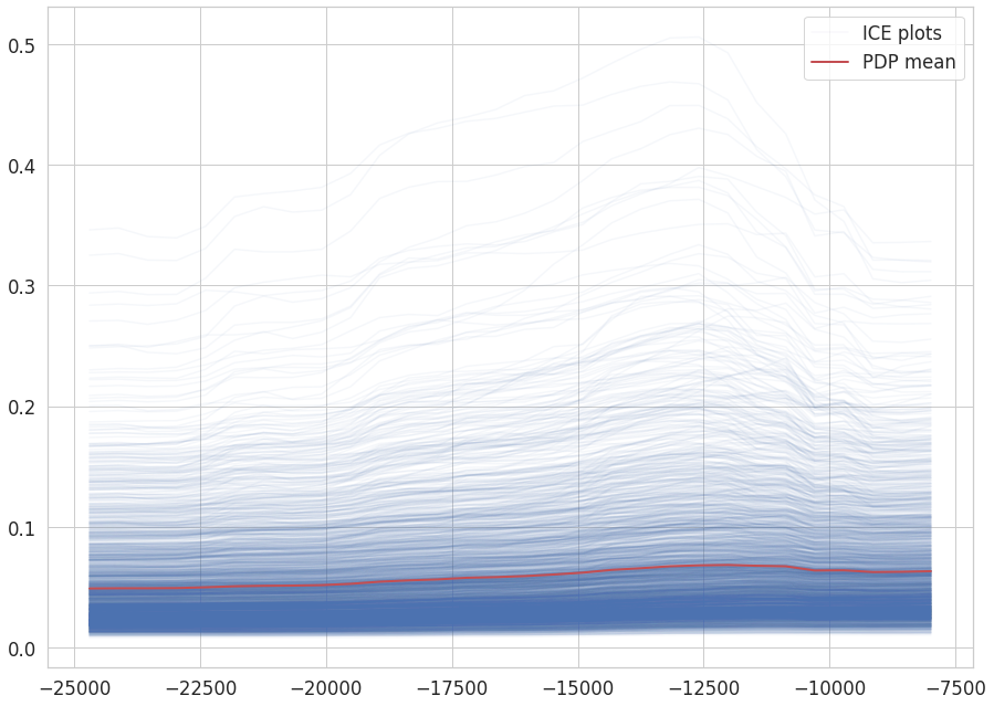
ICE shows the functional relationship between the predicted response and the feature separately for each instance. PDP averages the individual lines of an ICE plot.
Numeric features
For numeric features you can specify n_bins - number of bins into which the range of feature values is divided.
Calculate data for PDP plot manually:
[8]:
%%time

grid, ys, counts = automl.get_individual_pdp(test_data, feature_name='DAYS_BIRTH', n_bins=30)
100%|██████████| 30/30 [00:18<00:00, 1.63it/s]
CPU times: user 2min 2s, sys: 7.35 s, total: 2min 9s
Wall time: 18.4 s
[9]:
%%time

X = np.array([item.ravel() for item in ys]).T

plt.figure(figsize=(15, 11))
plt.plot(grid, X[0], alpha=0.05, color='m', label='ICE plots')
for i in range(1, X.shape[0]):
    plt.plot(grid, X[i], alpha=0.05, color='b')
plt.plot(grid, X.mean(axis=0), linewidth=2, color='r', label='PDP mean')
plt.legend()
plt.show()
CPU times: user 5.9 s, sys: 3.63 s, total: 9.53 s
Wall time: 2.46 s
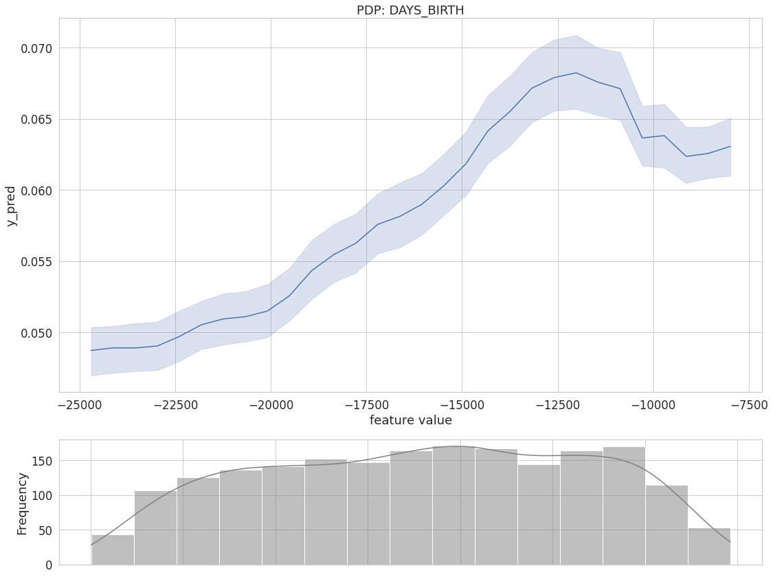
Built-in function:
[10]:
automl.plot_pdp(test_data, feature_name='DAYS_BIRTH')
100%|██████████| 30/30 [00:17<00:00, 1.67it/s]
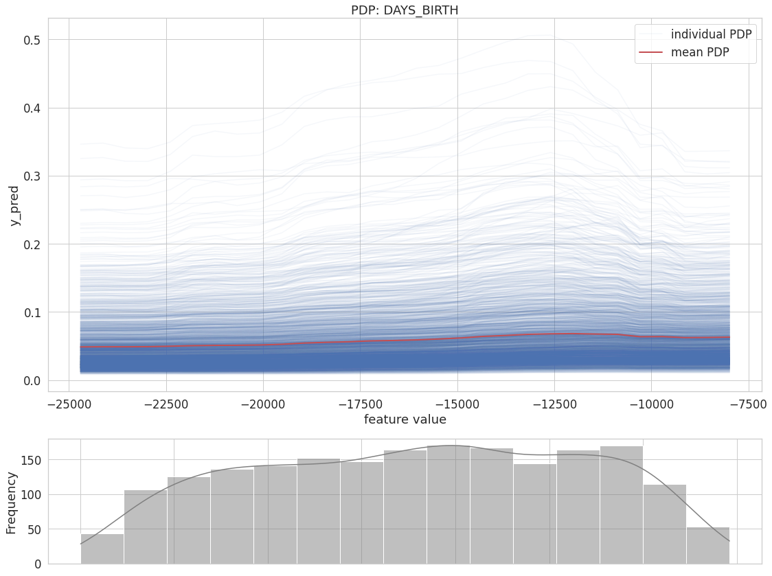
[11]:
automl.plot_pdp(test_data, feature_name='DAYS_BIRTH', individual=True)
100%|██████████| 30/30 [00:18<00:00, 1.63it/s]
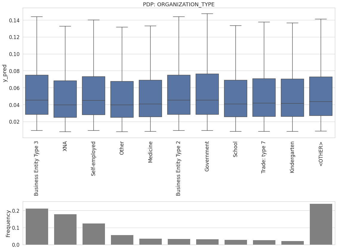
Categorical features
[12]:
%%time

automl.plot_pdp(test_data, feature_name='ORGANIZATION_TYPE')
100%|██████████| 10/10 [00:05<00:00, 1.69it/s]
CPU times: user 43.8 s, sys: 2.54 s, total: 46.4 s
Wall time: 6.87 s
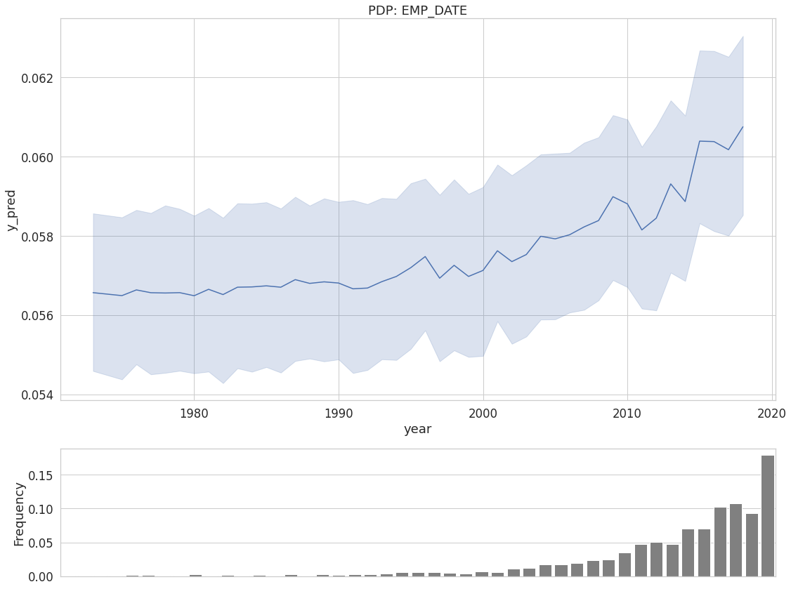
Datetime features
For datetime features you can specify groupby level, allowed values: year, month, dayofweek.
[13]:
%%time

automl.plot_pdp(test_data, feature_name='EMP_DATE', datetime_level='year')
100%|██████████| 45/45 [00:27<00:00, 1.63it/s]
CPU times: user 3min 2s, sys: 10.2 s, total: 3min 12s
Wall time: 29.4 s