Tutorial 6: Custom pipeline tutorial
![]()
Official LightAutoML github repository is here
Preparing
Step 1. Install LightAutoML
Uncomment if doesn’t clone repository by git. (ex.: colab, kaggle version)
[1]:
#! pip install -U lightautoml
Step 2. Import necessary libraries
[2]:
# Standard python libraries
import os
import time
import requests


# Installed libraries
import numpy as np
import pandas as pd
from sklearn.metrics import roc_auc_score
from sklearn.model_selection import train_test_split
import torch

# Imports from our package
from lightautoml.automl.base import AutoML
from lightautoml.ml_algo.boost_lgbm import BoostLGBM
from lightautoml.ml_algo.tuning.optuna import OptunaTuner
from lightautoml.pipelines.features.lgb_pipeline import LGBSimpleFeatures
from lightautoml.pipelines.ml.base import MLPipeline
from lightautoml.pipelines.selection.importance_based import ImportanceCutoffSelector, ModelBasedImportanceEstimator
from lightautoml.reader.base import PandasToPandasReader
from lightautoml.tasks import Task
from lightautoml.automl.blend import WeightedBlender
Step 3. Parameters
[3]:
N_THREADS = 8 # threads cnt for lgbm and linear models
N_FOLDS = 5 # folds cnt for AutoML
RANDOM_STATE = 42 # fixed random state for various reasons
TEST_SIZE = 0.2 # Test size for metric check
TARGET_NAME = 'TARGET' # Target column name
Step 4. Fix torch number of threads and numpy seed
[4]:
np.random.seed(RANDOM_STATE)
torch.set_num_threads(N_THREADS)
Step 5. Example data load
Load a dataset from the repository if doesn’t clone repository by git.
[5]:
DATASET_DIR = '../data/'
DATASET_NAME = 'sampled_app_train.csv'
DATASET_FULLNAME = os.path.join(DATASET_DIR, DATASET_NAME)
DATASET_URL = 'https://raw.githubusercontent.com/AILab-MLTools/LightAutoML/master/examples/data/sampled_app_train.csv'
[6]:
%%time

if not os.path.exists(DATASET_FULLNAME):
    os.makedirs(DATASET_DIR, exist_ok=True)

    dataset = requests.get(DATASET_URL).text
    with open(DATASET_FULLNAME, 'w') as output:
        output.write(dataset)
CPU times: user 28 µs, sys: 20 µs, total: 48 µs
Wall time: 64.4 µs
[7]:
%%time

data = pd.read_csv(DATASET_FULLNAME)
data.head()
CPU times: user 105 ms, sys: 14.5 ms, total: 119 ms
Wall time: 118 ms
[7]:
| SK_ID_CURR | TARGET | NAME_CONTRACT_TYPE | CODE_GENDER | FLAG_OWN_CAR | FLAG_OWN_REALTY | CNT_CHILDREN | AMT_INCOME_TOTAL | AMT_CREDIT | AMT_ANNUITY | ... | FLAG_DOCUMENT_18 | FLAG_DOCUMENT_19 | FLAG_DOCUMENT_20 | FLAG_DOCUMENT_21 | AMT_REQ_CREDIT_BUREAU_HOUR | AMT_REQ_CREDIT_BUREAU_DAY | AMT_REQ_CREDIT_BUREAU_WEEK | AMT_REQ_CREDIT_BUREAU_MON | AMT_REQ_CREDIT_BUREAU_QRT | AMT_REQ_CREDIT_BUREAU_YEAR | |
|---|---|---|---|---|---|---|---|---|---|---|---|---|---|---|---|---|---|---|---|---|---|
| 0 | 313802 | 0 | Cash loans | M | N | Y | 0 | 270000.0 | 327024.0 | 15372.0 | ... | 0 | 0 | 0 | 0 | 0.0 | 0.0 | 0.0 | 0.0 | 0.0 | 1.0 |
| 1 | 319656 | 0 | Cash loans | F | N | N | 0 | 108000.0 | 675000.0 | 19737.0 | ... | 0 | 0 | 0 | 0 | 0.0 | 0.0 | 0.0 | 0.0 | 0.0 | 0.0 |
| 2 | 207678 | 0 | Revolving loans | F | Y | Y | 2 | 112500.0 | 270000.0 | 13500.0 | ... | 0 | 0 | 0 | 0 | 0.0 | 0.0 | 0.0 | 0.0 | 0.0 | 1.0 |
| 3 | 381593 | 0 | Cash loans | F | N | N | 1 | 67500.0 | 142200.0 | 9630.0 | ... | 0 | 0 | 0 | 0 | 0.0 | 0.0 | 0.0 | 0.0 | 0.0 | 4.0 |
| 4 | 258153 | 0 | Cash loans | F | Y | Y | 0 | 337500.0 | 1483231.5 | 46570.5 | ... | 0 | 0 | 0 | 0 | 0.0 | 0.0 | 0.0 | 2.0 | 0.0 | 0.0 |
5 rows × 122 columns
Step 6. (Optional) Some user feature preparation
Cell below shows some user feature preparations to create task more difficult (this block can be omitted if you don’t want to change the initial data):
[8]:
%%time

data['BIRTH_DATE'] = (np.datetime64('2018-01-01') + data['DAYS_BIRTH'].astype(np.dtype('timedelta64[D]'))).astype(str)
data['EMP_DATE'] = (np.datetime64('2018-01-01') + np.clip(data['DAYS_EMPLOYED'], None, 0).astype(np.dtype('timedelta64[D]'))
                    ).astype(str)

data['constant'] = 1
data['allnan'] = np.nan

data['report_dt'] = np.datetime64('2018-01-01')

data.drop(['DAYS_BIRTH', 'DAYS_EMPLOYED'], axis=1, inplace=True)
CPU times: user 108 ms, sys: 4.5 ms, total: 113 ms
Wall time: 111 ms
Step 7. (Optional) Data splitting for train-test
Block below can be omitted if you are going to train model only or you have specific train and test files:
[9]:
%%time

train_data, test_data = train_test_split(data,
                                         test_size=TEST_SIZE,
                                         stratify=data[TARGET_NAME],
                                         random_state=RANDOM_STATE)
print('Data splitted. Parts sizes: train_data = {}, test_data = {}'
              .format(train_data.shape, test_data.shape))
Data splitted. Parts sizes: train_data = (8000, 125), test_data = (2000, 125)
CPU times: user 7.85 ms, sys: 3.89 ms, total: 11.7 ms
Wall time: 10.1 ms
[10]:
train_data.head()
[10]:
| SK_ID_CURR | TARGET | NAME_CONTRACT_TYPE | CODE_GENDER | FLAG_OWN_CAR | FLAG_OWN_REALTY | CNT_CHILDREN | AMT_INCOME_TOTAL | AMT_CREDIT | AMT_ANNUITY | ... | AMT_REQ_CREDIT_BUREAU_DAY | AMT_REQ_CREDIT_BUREAU_WEEK | AMT_REQ_CREDIT_BUREAU_MON | AMT_REQ_CREDIT_BUREAU_QRT | AMT_REQ_CREDIT_BUREAU_YEAR | BIRTH_DATE | EMP_DATE | constant | allnan | report_dt | |
|---|---|---|---|---|---|---|---|---|---|---|---|---|---|---|---|---|---|---|---|---|---|
| 6444 | 112261 | 0 | Cash loans | F | N | N | 1 | 90000.0 | 640080.0 | 31261.5 | ... | 0.0 | 0.0 | 0.0 | 1.0 | 0.0 | 1985-06-28 | 2012-06-21 | 1 | NaN | 2018-01-01 |
| 3586 | 115058 | 0 | Cash loans | F | N | Y | 0 | 180000.0 | 239850.0 | 23850.0 | ... | 0.0 | 0.0 | 0.0 | 0.0 | 3.0 | 1953-12-27 | 2018-01-01 | 1 | NaN | 2018-01-01 |
| 9349 | 326623 | 0 | Cash loans | F | N | Y | 0 | 112500.0 | 337500.0 | 31086.0 | ... | 0.0 | 0.0 | 0.0 | 0.0 | 2.0 | 1975-06-21 | 2016-06-17 | 1 | NaN | 2018-01-01 |
| 7734 | 191976 | 0 | Cash loans | M | Y | Y | 1 | 67500.0 | 135000.0 | 9018.0 | ... | NaN | NaN | NaN | NaN | NaN | 1988-04-27 | 2009-06-05 | 1 | NaN | 2018-01-01 |
| 2174 | 281519 | 0 | Revolving loans | F | N | Y | 0 | 67500.0 | 202500.0 | 10125.0 | ... | 0.0 | 0.0 | 0.0 | 0.0 | 2.0 | 1975-06-13 | 1997-01-22 | 1 | NaN | 2018-01-01 |
5 rows × 125 columns
AutoML creation
Step 1. Create Task and PandasReader
[11]:
%%time

task = Task('binary')
reader = PandasToPandasReader(task, cv=N_FOLDS, random_state=RANDOM_STATE)
CPU times: user 4.03 ms, sys: 25 µs, total: 4.05 ms
Wall time: 2.99 ms
Step 2. Create feature selector (if necessary)
[12]:
%%time

model0 = BoostLGBM(
    default_params={'learning_rate': 0.05, 'num_leaves': 64, 'seed': 42, 'num_threads': N_THREADS}
)
pipe0 = LGBSimpleFeatures()
mbie = ModelBasedImportanceEstimator()
selector = ImportanceCutoffSelector(pipe0, model0, mbie, cutoff=0)
Copying TaskTimer may affect the parent PipelineTimer, so copy will create new unlimited TaskTimer
CPU times: user 0 ns, sys: 1.91 ms, total: 1.91 ms
Wall time: 1.56 ms
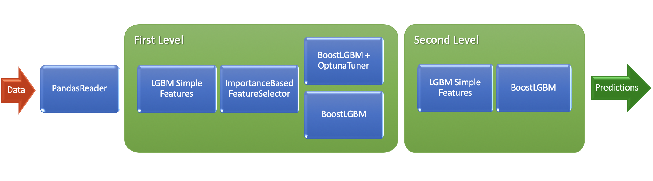
Step 3.1. Create 1st level ML pipeline for AutoML
Our first level ML pipeline: - Simple features for gradient boosting built on selected features (using step 2) - 2 different models: * LightGBM with params tuning (using OptunaTuner) * LightGBM with heuristic params
[13]:
%%time

pipe = LGBSimpleFeatures()

params_tuner1 = OptunaTuner(n_trials=20, timeout=30) # stop after 20 iterations or after 30 seconds
model1 = BoostLGBM(
    default_params={'learning_rate': 0.05, 'num_leaves': 128, 'seed': 1, 'num_threads': N_THREADS}
)
model2 = BoostLGBM(
    default_params={'learning_rate': 0.025, 'num_leaves': 64, 'seed': 2, 'num_threads': N_THREADS}
)

pipeline_lvl1 = MLPipeline([
    (model1, params_tuner1),
    model2
], pre_selection=selector, features_pipeline=pipe, post_selection=None)
CPU times: user 51 µs, sys: 37 µs, total: 88 µs
Wall time: 96.8 µs
Step 3.2. Create 2nd level ML pipeline for AutoML
Our second level ML pipeline: - Using simple features as well, but now it will be Out-Of-Fold (OOF) predictions of algos from 1st level - Only one LGBM model without params tuning - Without feature selection on this stage because we want to use all OOFs here
[14]:
%%time

pipe1 = LGBSimpleFeatures()

model = BoostLGBM(
    default_params={'learning_rate': 0.05, 'num_leaves': 64, 'max_bin': 1024, 'seed': 3, 'num_threads': N_THREADS},
    freeze_defaults=True
)

pipeline_lvl2 = MLPipeline([model], pre_selection=None, features_pipeline=pipe1, post_selection=None)
CPU times: user 41 µs, sys: 29 µs, total: 70 µs
Wall time: 81.5 µs
Step 4. Create AutoML pipeline
AutoML pipeline consist of: - Reader for data preparation - First level ML pipeline (as built in step 3.1) - Second level ML pipeline (as built in step 3.2) - Skip_conn = False equals here “not to use initial features on the second level pipeline”
[15]:
%%time

automl = AutoML(reader, [
    [pipeline_lvl1],
    [pipeline_lvl2],
], skip_conn=False)
CPU times: user 35 µs, sys: 24 µs, total: 59 µs
Wall time: 73.7 µs
Step 5. Train AutoML on loaded data
In cell below we train AutoML with target column TARGET to receive fitted model and OOF predictions:
[16]:
%%time

oof_pred = automl.fit_predict(train_data, roles={'target': TARGET_NAME})
print('oof_pred:\n{}\nShape = {}'.format(oof_pred, oof_pred.shape))
[LightGBM] [Warning] seed is set=42, random_state=42 will be ignored. Current value: seed=42
[LightGBM] [Warning] seed is set=1, random_state=42 will be ignored. Current value: seed=1
[LightGBM] [Warning] seed is set=1, random_state=42 will be ignored. Current value: seed=1
[LightGBM] [Warning] seed is set=1, random_state=42 will be ignored. Current value: seed=1
[LightGBM] [Warning] seed is set=1, random_state=42 will be ignored. Current value: seed=1
[LightGBM] [Warning] seed is set=1, random_state=42 will be ignored. Current value: seed=1
[LightGBM] [Warning] seed is set=1, random_state=42 will be ignored. Current value: seed=1
[LightGBM] [Warning] seed is set=1, random_state=42 will be ignored. Current value: seed=1
[LightGBM] [Warning] seed is set=1, random_state=42 will be ignored. Current value: seed=1
[LightGBM] [Warning] seed is set=1, random_state=42 will be ignored. Current value: seed=1
[LightGBM] [Warning] seed is set=1, random_state=42 will be ignored. Current value: seed=1
[LightGBM] [Warning] seed is set=1, random_state=42 will be ignored. Current value: seed=1
[LightGBM] [Warning] seed is set=1, random_state=42 will be ignored. Current value: seed=1
[LightGBM] [Warning] seed is set=1, random_state=42 will be ignored. Current value: seed=1
[LightGBM] [Warning] seed is set=1, random_state=42 will be ignored. Current value: seed=1
[LightGBM] [Warning] seed is set=1, random_state=42 will be ignored. Current value: seed=1
[LightGBM] [Warning] seed is set=1, random_state=42 will be ignored. Current value: seed=1
[LightGBM] [Warning] seed is set=1, random_state=42 will be ignored. Current value: seed=1
[LightGBM] [Warning] seed is set=1, random_state=42 will be ignored. Current value: seed=1
[LightGBM] [Warning] seed is set=1, random_state=42 will be ignored. Current value: seed=1
[LightGBM] [Warning] seed is set=1, random_state=42 will be ignored. Current value: seed=1
[LightGBM] [Warning] seed is set=1, random_state=42 will be ignored. Current value: seed=1
[LightGBM] [Warning] seed is set=1, random_state=42 will be ignored. Current value: seed=1
[LightGBM] [Warning] seed is set=1, random_state=42 will be ignored. Current value: seed=1
[LightGBM] [Warning] seed is set=1, random_state=42 will be ignored. Current value: seed=1
[LightGBM] [Warning] seed is set=1, random_state=42 will be ignored. Current value: seed=1
[LightGBM] [Warning] seed is set=2, random_state=42 will be ignored. Current value: seed=2
[LightGBM] [Warning] seed is set=2, random_state=42 will be ignored. Current value: seed=2
[LightGBM] [Warning] seed is set=2, random_state=42 will be ignored. Current value: seed=2
[LightGBM] [Warning] seed is set=2, random_state=42 will be ignored. Current value: seed=2
[LightGBM] [Warning] seed is set=2, random_state=42 will be ignored. Current value: seed=2
[LightGBM] [Warning] seed is set=3, random_state=42 will be ignored. Current value: seed=3
[LightGBM] [Warning] seed is set=3, random_state=42 will be ignored. Current value: seed=3
[LightGBM] [Warning] seed is set=3, random_state=42 will be ignored. Current value: seed=3
[LightGBM] [Warning] seed is set=3, random_state=42 will be ignored. Current value: seed=3
[LightGBM] [Warning] seed is set=3, random_state=42 will be ignored. Current value: seed=3
oof_pred:
array([[0.07027727],
       [0.06983411],
       [0.06983411],
       ...,
       [0.04349083],
       [0.09716105],
       [0.12494681]], dtype=float32)
Shape = (8000, 1)
CPU times: user 4min 23s, sys: 2.63 s, total: 4min 26s
Wall time: 37.3 s
Step 6. Analyze fitted model
Below we analyze feature importances of different algos:
[17]:
print('Feature importances of selector:\n{}'
              .format(selector.get_features_score()))
print('=' * 70)

print('Feature importances of top level algorithm:\n{}'
              .format(automl.levels[-1][0].ml_algos[0].get_features_score()))
print('=' * 70)

print('Feature importances of lowest level algorithm - model 0:\n{}'
              .format(automl.levels[0][0].ml_algos[0].get_features_score()))
print('=' * 70)

print('Feature importances of lowest level algorithm - model 1:\n{}'
              .format(automl.levels[0][0].ml_algos[1].get_features_score()))
print('=' * 70)
Feature importances of selector:
EXT_SOURCE_3              1029.681686
EXT_SOURCE_2               894.265428
BIRTH_DATE                 537.081401
EXT_SOURCE_1               424.764621
DAYS_LAST_PHONE_CHANGE     262.583100
                             ...
FLAG_DOCUMENT_16             0.000000
FLAG_DOCUMENT_14             0.000000
FLAG_DOCUMENT_13             0.000000
FLAG_DOCUMENT_11             0.000000
FLAG_PHONE                   0.000000
Length: 110, dtype: float64
======================================================================
Feature importances of top level algorithm:
Lvl_0_Pipe_0_Mod_0_LightGBM_prediction_0    2546.473691
Lvl_0_Pipe_0_Mod_1_LightGBM_prediction_0    1686.589227
dtype: float64
======================================================================
Feature importances of lowest level algorithm - model 0:
EXT_SOURCE_2                  1500.371550
EXT_SOURCE_3                  1382.049802
dtdiff__BIRTH_DATE             714.069627
EXT_SOURCE_1                   573.079861
DAYS_REGISTRATION              461.927863
                                 ...
ord__HOUSETYPE_MODE              1.985318
ELEVATORS_MEDI                   1.862320
FLAG_DOCUMENT_6                  0.000000
REG_REGION_NOT_WORK_REGION       0.000000
ord__FLAG_OWN_CAR                0.000000
Length: 85, dtype: float64
======================================================================
Feature importances of lowest level algorithm - model 1:
EXT_SOURCE_3                   2666.270588
EXT_SOURCE_2                   2425.430385
dtdiff__BIRTH_DATE             1607.440484
DAYS_REGISTRATION              1217.128893
SK_ID_CURR                     1136.992744
                                  ...
LIVE_REGION_NOT_WORK_REGION       9.561320
ord__EMERGENCYSTATE_MODE          7.256624
REG_REGION_NOT_WORK_REGION        5.843864
ord__NAME_CONTRACT_TYPE           3.890026
FLAG_DOCUMENT_6                   3.523548
Length: 85, dtype: float64
======================================================================
Step 7. Predict to test data and check scores
[18]:
%%time

test_pred = automl.predict(test_data)
print('Prediction for test data:\n{}\nShape = {}'
              .format(test_pred, test_pred.shape))

print('Check scores...')
print('OOF score: {}'.format(roc_auc_score(train_data[TARGET_NAME].values, oof_pred.data[:, 0])))
print('TEST score: {}'.format(roc_auc_score(test_data[TARGET_NAME].values, test_pred.data[:, 0])))
Prediction for test data:
array([[0.060448  ],
       [0.07832611],
       [0.05339179],
       ...,
       [0.06192666],
       [0.07732402],
       [0.20730501]], dtype=float32)
Shape = (2000, 1)
Check scores...
OOF score: 0.6979918272484156
TEST score: 0.7158254076086956
CPU times: user 421 ms, sys: 11.6 ms, total: 433 ms
Wall time: 103 ms