Tutorial 3: SQL data source
![]()
Official LightAutoML github repository is here
Preparing
Step 1. Install LightAutoML
Uncomment if doesn’t clone repository by git. (ex.: colab, kaggle version)
[1]:
#! pip install -U lightautoml
Step 2. Import necessary libraries
[2]:
# Standard python libraries
import os
import time
import requests
# Installed libraries
import numpy as np
import pandas as pd
from sklearn.metrics import roc_auc_score
from sklearn.model_selection import train_test_split
import torch

# Imports from our package
import gensim
from lightautoml.automl.presets.tabular_presets import TabularAutoML, TabularUtilizedAutoML
from lightautoml.dataset.roles import DatetimeRole
from lightautoml.tasks import Task
Step 3. Parameters
[3]:
N_THREADS = 8 # threads cnt for lgbm and linear models
N_FOLDS = 5 # folds cnt for AutoML
RANDOM_STATE = 42 # fixed random state for various reasons
TEST_SIZE = 0.2 # Test size for metric check
TIMEOUT = 300 # Time in seconds for automl run
TARGET_NAME = 'TARGET' # Target column name
Step 4. Fix torch number of threads and numpy seed
[4]:
np.random.seed(RANDOM_STATE)
torch.set_num_threads(N_THREADS)
Step 5. Example data load
Load a dataset from the repository if doesn’t clone repository by git.
[5]:
DATASET_DIR = '../data/'
DATASET_NAME = 'sampled_app_train.csv'
DATASET_FULLNAME = os.path.join(DATASET_DIR, DATASET_NAME)
DATASET_URL = 'https://raw.githubusercontent.com/AILab-MLTools/LightAutoML/master/examples/data/sampled_app_train.csv'
[6]:
%%time

if not os.path.exists(DATASET_FULLNAME):
    os.makedirs(DATASET_DIR, exist_ok=True)

    dataset = requests.get(DATASET_URL).text
    with open(DATASET_FULLNAME, 'w') as output:
        output.write(dataset)
CPU times: user 29 µs, sys: 20 µs, total: 49 µs
Wall time: 68.4 µs
[7]:
%%time

data = pd.read_csv(DATASET_FULLNAME)
data.head()
CPU times: user 104 ms, sys: 19.8 ms, total: 123 ms
Wall time: 122 ms
[7]:
| SK_ID_CURR | TARGET | NAME_CONTRACT_TYPE | CODE_GENDER | FLAG_OWN_CAR | FLAG_OWN_REALTY | CNT_CHILDREN | AMT_INCOME_TOTAL | AMT_CREDIT | AMT_ANNUITY | ... | FLAG_DOCUMENT_18 | FLAG_DOCUMENT_19 | FLAG_DOCUMENT_20 | FLAG_DOCUMENT_21 | AMT_REQ_CREDIT_BUREAU_HOUR | AMT_REQ_CREDIT_BUREAU_DAY | AMT_REQ_CREDIT_BUREAU_WEEK | AMT_REQ_CREDIT_BUREAU_MON | AMT_REQ_CREDIT_BUREAU_QRT | AMT_REQ_CREDIT_BUREAU_YEAR | |
|---|---|---|---|---|---|---|---|---|---|---|---|---|---|---|---|---|---|---|---|---|---|
| 0 | 313802 | 0 | Cash loans | M | N | Y | 0 | 270000.0 | 327024.0 | 15372.0 | ... | 0 | 0 | 0 | 0 | 0.0 | 0.0 | 0.0 | 0.0 | 0.0 | 1.0 |
| 1 | 319656 | 0 | Cash loans | F | N | N | 0 | 108000.0 | 675000.0 | 19737.0 | ... | 0 | 0 | 0 | 0 | 0.0 | 0.0 | 0.0 | 0.0 | 0.0 | 0.0 |
| 2 | 207678 | 0 | Revolving loans | F | Y | Y | 2 | 112500.0 | 270000.0 | 13500.0 | ... | 0 | 0 | 0 | 0 | 0.0 | 0.0 | 0.0 | 0.0 | 0.0 | 1.0 |
| 3 | 381593 | 0 | Cash loans | F | N | N | 1 | 67500.0 | 142200.0 | 9630.0 | ... | 0 | 0 | 0 | 0 | 0.0 | 0.0 | 0.0 | 0.0 | 0.0 | 4.0 |
| 4 | 258153 | 0 | Cash loans | F | Y | Y | 0 | 337500.0 | 1483231.5 | 46570.5 | ... | 0 | 0 | 0 | 0 | 0.0 | 0.0 | 0.0 | 2.0 | 0.0 | 0.0 |
5 rows × 122 columns
Step 6. (Optional) Some user feature preparation
Cell below shows some user feature preparations to create task more difficult (this block can be omitted if you don’t want to change the initial data):
[8]:
%%time

data['BIRTH_DATE'] = (np.datetime64('2018-01-01') + data['DAYS_BIRTH'].astype(np.dtype('timedelta64[D]'))).astype(str)
data['EMP_DATE'] = (np.datetime64('2018-01-01') + np.clip(data['DAYS_EMPLOYED'], None, 0).astype(np.dtype('timedelta64[D]'))
                    ).astype(str)

data['constant'] = 1
data['allnan'] = np.nan

data['report_dt'] = np.datetime64('2018-01-01')

data.drop(['DAYS_BIRTH', 'DAYS_EMPLOYED'], axis=1, inplace=True)
CPU times: user 105 ms, sys: 8.82 ms, total: 114 ms
Wall time: 112 ms
Step 7. (Optional) Data splitting for train-test
Block below can be omitted if you are going to train model only or you have specific train and test files:
[9]:
%%time

train_data, test_data = train_test_split(data,
                                         test_size=TEST_SIZE,
                                         stratify=data[TARGET_NAME],
                                         random_state=RANDOM_STATE)
print('Data splitted. Parts sizes: train_data = {}, test_data = {}'
              .format(train_data.shape, test_data.shape))
Data splitted. Parts sizes: train_data = (8000, 125), test_data = (2000, 125)
CPU times: user 11.2 ms, sys: 0 ns, total: 11.2 ms
Wall time: 9.95 ms
[10]:
train_data.head()
[10]:
| SK_ID_CURR | TARGET | NAME_CONTRACT_TYPE | CODE_GENDER | FLAG_OWN_CAR | FLAG_OWN_REALTY | CNT_CHILDREN | AMT_INCOME_TOTAL | AMT_CREDIT | AMT_ANNUITY | ... | AMT_REQ_CREDIT_BUREAU_DAY | AMT_REQ_CREDIT_BUREAU_WEEK | AMT_REQ_CREDIT_BUREAU_MON | AMT_REQ_CREDIT_BUREAU_QRT | AMT_REQ_CREDIT_BUREAU_YEAR | BIRTH_DATE | EMP_DATE | constant | allnan | report_dt | |
|---|---|---|---|---|---|---|---|---|---|---|---|---|---|---|---|---|---|---|---|---|---|
| 6444 | 112261 | 0 | Cash loans | F | N | N | 1 | 90000.0 | 640080.0 | 31261.5 | ... | 0.0 | 0.0 | 0.0 | 1.0 | 0.0 | 1985-06-28 | 2012-06-21 | 1 | NaN | 2018-01-01 |
| 3586 | 115058 | 0 | Cash loans | F | N | Y | 0 | 180000.0 | 239850.0 | 23850.0 | ... | 0.0 | 0.0 | 0.0 | 0.0 | 3.0 | 1953-12-27 | 2018-01-01 | 1 | NaN | 2018-01-01 |
| 9349 | 326623 | 0 | Cash loans | F | N | Y | 0 | 112500.0 | 337500.0 | 31086.0 | ... | 0.0 | 0.0 | 0.0 | 0.0 | 2.0 | 1975-06-21 | 2016-06-17 | 1 | NaN | 2018-01-01 |
| 7734 | 191976 | 0 | Cash loans | M | Y | Y | 1 | 67500.0 | 135000.0 | 9018.0 | ... | NaN | NaN | NaN | NaN | NaN | 1988-04-27 | 2009-06-05 | 1 | NaN | 2018-01-01 |
| 2174 | 281519 | 0 | Revolving loans | F | N | Y | 0 | 67500.0 | 202500.0 | 10125.0 | ... | 0.0 | 0.0 | 0.0 | 0.0 | 2.0 | 1975-06-13 | 1997-01-22 | 1 | NaN | 2018-01-01 |
5 rows × 125 columns
Step 8. (Optional) Reading data from SqlDataSource
Preparing datasets as SQLite data bases
[11]:
import sqlite3 as sql

for _fname in ('train.db', 'test.db'):
    if os.path.exists(_fname):
        os.remove(_fname)

train_db = sql.connect('train.db')
train_data.to_sql('data', train_db)

test_db = sql.connect('test.db')
test_data.to_sql('data', test_db)
Using dataset wrapper for a connection
[12]:
from lightautoml.reader.tabular_batch_generator import SqlDataSource

# train_data is replaced with a wrapper for an SQLAlchemy connection
# Wrapper requires SQLAlchemy connection string and query to obtain data from
train_data = SqlDataSource('sqlite:///train.db', 'select * from data', index='index')
test_data = SqlDataSource('sqlite:///test.db', 'select * from data', index='index')
AutoML preset usage
Step 1. Create Task
[13]:
%%time

task = Task('binary', )
CPU times: user 6.11 ms, sys: 1.41 ms, total: 7.52 ms
Wall time: 5.65 ms
Step 2. Setup columns roles
Roles setup here set target column and base date, which is used to calculate date differences:
[14]:
%%time

roles = {'target': TARGET_NAME,
         DatetimeRole(base_date=True, seasonality=(), base_feats=False): 'report_dt',
         }
CPU times: user 48 µs, sys: 32 µs, total: 80 µs
Wall time: 95.1 µs
Step 3. Create AutoML from preset
To create AutoML model here we use TabularAutoML preset, which looks like:
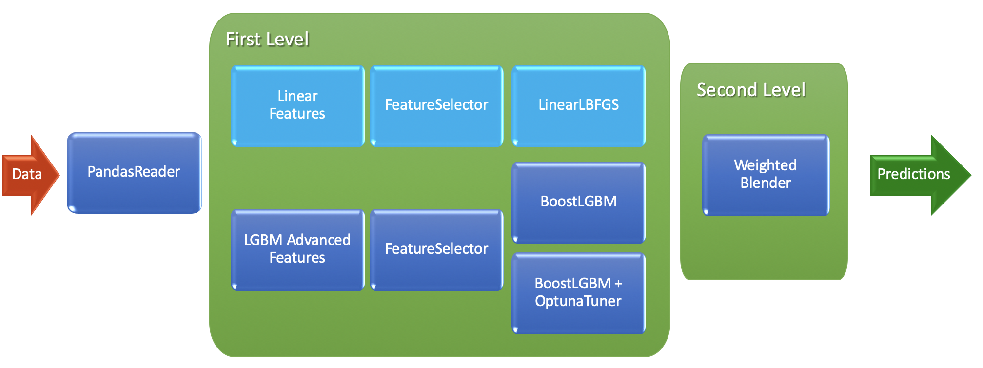
All params we set above can be send inside preset to change its configuration:
[15]:
%%time

automl = TabularAutoML(task = task,
                       timeout = TIMEOUT,
                       general_params = {'nested_cv': False, 'use_algos': [['linear_l2', 'lgb', 'lgb_tuned']]},
                       reader_params = {'cv': N_FOLDS, 'random_state': RANDOM_STATE},
                       tuning_params = {'max_tuning_iter': 20, 'max_tuning_time': 30},
                       lgb_params = {'default_params': {'num_threads': N_THREADS}})
oof_pred = automl.fit_predict(train_data, roles = roles)
print('oof_pred:\n{}\nShape = {}'.format(oof_pred, oof_pred.shape))
oof_pred:
array([[0.0226106 ],
       [0.02359573],
       [0.02438388],
       ...,
       [0.02287533],
       [0.15669319],
       [0.08664417]], dtype=float32)
Shape = (8000, 1)
CPU times: user 4min 19s, sys: 3.59 s, total: 4min 23s
Wall time: 1min 11s
Step 4. Predict to test data and check scores
[16]:
%%time

test_pred = automl.predict(test_data)
print('Prediction for test data:\n{}\nShape = {}'
              .format(test_pred, test_pred.shape))

print('Check scores...')
print('OOF score: {}'.format(roc_auc_score(train_data.data[TARGET_NAME].values, oof_pred.data[:, 0])))
print('TEST score: {}'.format(roc_auc_score(test_data.data[TARGET_NAME].values, test_pred.data[:, 0])))
Prediction for test data:
array([[0.05828221],
       [0.07749337],
       [0.02520473],
       ...,
       [0.05070161],
       [0.0373171 ],
       [0.23640296]], dtype=float32)
Shape = (2000, 1)
Check scores...
OOF score: 0.7500913646530726
TEST score: 0.7331657608695653
CPU times: user 1.05 s, sys: 4.05 ms, total: 1.06 s
Wall time: 449 ms
Step 5. Create AutoML with time utilization
Below we are going to create specific AutoML preset for TIMEOUT utilization (try to spend it as much as possible):
[20]:
%%time

automl = TabularUtilizedAutoML(task = task,
                       timeout = TIMEOUT,
                       general_params = {'nested_cv': False, 'use_algos': [['linear_l2', 'lgb', 'lgb_tuned']]},
                       reader_params = {'cv': N_FOLDS, 'random_state': RANDOM_STATE},
                       tuning_params = {'max_tuning_iter': 20, 'max_tuning_time': 30},
                       lgb_params = {'default_params': {'num_threads': N_THREADS}})
oof_pred = automl.fit_predict(train_data, roles = roles)
print('oof_pred:\n{}\nShape = {}'.format(oof_pred, oof_pred.shape))
oof_pred:
array([[0.0343032 ],
       [0.01933593],
       [0.02276292],
       ...,
       [0.02349434],
       [0.17084229],
       [0.09522362]], dtype=float32)
Shape = (8000, 1)
CPU times: user 16min 54s, sys: 12.3 s, total: 17min 6s
Wall time: 4min 29s
Step 6. Predict to test data and check scores for utilized automl
[21]:
%%time

test_pred = automl.predict(test_data)
print('Prediction for test data:\n{}\nShape = {}'
              .format(test_pred, test_pred.shape))

print('Check scores...')
print('OOF score: {}'.format(roc_auc_score(train_data.data[TARGET_NAME].values, oof_pred.data[:, 0])))
print('TEST score: {}'.format(roc_auc_score(test_data.data[TARGET_NAME].values, test_pred.data[:, 0])))
Prediction for test data:
array([[0.05981494],
       [0.07601136],
       [0.02678316],
       ...,
       [0.04721078],
       [0.03855655],
       [0.19377196]], dtype=float32)
Shape = (2000, 1)
Check scores...
OOF score: 0.7586795357421285
TEST score: 0.730679347826087
CPU times: user 2.99 s, sys: 64.1 ms, total: 3.05 s
Wall time: 1.21 s
[ ]: