Tutorial 1: Basics
![]()
Official LightAutoML github repository is here
In this tutorial you will learn how to: * run LightAutoML training on tabular data * obtain feature importances and reports * configure resource usage in LightAutoML
0. Prerequisites
0.0. install LightAutoML
[1]:
#!pip install -U lightautoml
0.1. Import libraries
Here we will import the libraries we use in this kernel: - Standard python libraries for timing, working with OS and HTTP requests etc. - Essential python DS libraries like numpy, pandas, scikit-learn and torch (the last we will use in the next cell) - LightAutoML modules: presets for AutoML, task and report generation module
[1]:
import warnings
warnings.simplefilter(action='ignore', category=FutureWarning)
[1]:
# Standard python libraries
import os
import requests

# Essential DS libraries
import numpy as np
import pandas as pd
from sklearn.metrics import roc_auc_score
from sklearn.model_selection import train_test_split
import torch

# LightAutoML presets, task and report generation
from lightautoml.automl.presets.tabular_presets import TabularAutoML, TabularUtilizedAutoML
from lightautoml.tasks import Task
from lightautoml.report.report_deco import ReportDeco, ReportDecoUtilized
from lightautoml.addons.tabular_interpretation import SSWARM
0.2. Constants
Here we setup some parameters to use in the kernel: - N_THREADS - number of vCPUs for LightAutoML model creation - N_FOLDS - number of folds in LightAutoML inner CV - RANDOM_STATE - random seed for better reproducibility - TEST_SIZE - houldout data part size - TIMEOUT - limit in seconds for model to train - TARGET_NAME - target column name in dataset
[2]:
N_THREADS = 4
N_FOLDS = 5
RANDOM_STATE = 42
TEST_SIZE = 0.2
TIMEOUT = 300
TARGET_NAME = 'TARGET'
[3]:
DATASET_DIR = '../data/'
DATASET_NAME = 'sampled_app_train.csv'
DATASET_FULLNAME = os.path.join(DATASET_DIR, DATASET_NAME)
DATASET_URL = 'https://raw.githubusercontent.com/AILab-MLTools/LightAutoML/master/examples/data/sampled_app_train.csv'
0.3. Imported models setup
For better reproducibility fix numpy random seed with max number of threads for Torch (which usually try to use all the threads on server):
[4]:
np.random.seed(RANDOM_STATE)
torch.set_num_threads(N_THREADS)
0.4. Data loading
Let’s check the data we have:
[5]:
if not os.path.exists(DATASET_FULLNAME):
    os.makedirs(DATASET_DIR, exist_ok=True)

    dataset = requests.get(DATASET_URL).text
    with open(DATASET_FULLNAME, 'w') as output:
        output.write(dataset)
[6]:
data = pd.read_csv(DATASET_DIR + DATASET_NAME)
data.head()
[6]:
| SK_ID_CURR | TARGET | NAME_CONTRACT_TYPE | CODE_GENDER | FLAG_OWN_CAR | FLAG_OWN_REALTY | CNT_CHILDREN | AMT_INCOME_TOTAL | AMT_CREDIT | AMT_ANNUITY | ... | FLAG_DOCUMENT_18 | FLAG_DOCUMENT_19 | FLAG_DOCUMENT_20 | FLAG_DOCUMENT_21 | AMT_REQ_CREDIT_BUREAU_HOUR | AMT_REQ_CREDIT_BUREAU_DAY | AMT_REQ_CREDIT_BUREAU_WEEK | AMT_REQ_CREDIT_BUREAU_MON | AMT_REQ_CREDIT_BUREAU_QRT | AMT_REQ_CREDIT_BUREAU_YEAR | |
|---|---|---|---|---|---|---|---|---|---|---|---|---|---|---|---|---|---|---|---|---|---|
| 0 | 313802 | 0 | Cash loans | M | N | Y | 0 | 270000.0 | 327024.0 | 15372.0 | ... | 0 | 0 | 0 | 0 | 0.0 | 0.0 | 0.0 | 0.0 | 0.0 | 1.0 |
| 1 | 319656 | 0 | Cash loans | F | N | N | 0 | 108000.0 | 675000.0 | 19737.0 | ... | 0 | 0 | 0 | 0 | 0.0 | 0.0 | 0.0 | 0.0 | 0.0 | 0.0 |
| 2 | 207678 | 0 | Revolving loans | F | Y | Y | 2 | 112500.0 | 270000.0 | 13500.0 | ... | 0 | 0 | 0 | 0 | 0.0 | 0.0 | 0.0 | 0.0 | 0.0 | 1.0 |
| 3 | 381593 | 0 | Cash loans | F | N | N | 1 | 67500.0 | 142200.0 | 9630.0 | ... | 0 | 0 | 0 | 0 | 0.0 | 0.0 | 0.0 | 0.0 | 0.0 | 4.0 |
| 4 | 258153 | 0 | Cash loans | F | Y | Y | 0 | 337500.0 | 1483231.5 | 46570.5 | ... | 0 | 0 | 0 | 0 | 0.0 | 0.0 | 0.0 | 2.0 | 0.0 | 0.0 |
5 rows × 122 columns
[7]:
data.shape
[7]:
(10000, 122)
0.5. Data splitting for train-holdout
As we have only one file with target values, we can split it into 80%-20% for holdout usage:
[8]:
train_data, test_data = train_test_split(
    data,
    test_size=TEST_SIZE,
    stratify=data[TARGET_NAME],
    random_state=RANDOM_STATE
)

print(f'Data is splitted. Parts sizes: train_data = {train_data.shape}, test_data = {test_data.shape}')

train_data.head()
Data is splitted. Parts sizes: train_data = (8000, 122), test_data = (2000, 122)
[8]:
| SK_ID_CURR | TARGET | NAME_CONTRACT_TYPE | CODE_GENDER | FLAG_OWN_CAR | FLAG_OWN_REALTY | CNT_CHILDREN | AMT_INCOME_TOTAL | AMT_CREDIT | AMT_ANNUITY | ... | FLAG_DOCUMENT_18 | FLAG_DOCUMENT_19 | FLAG_DOCUMENT_20 | FLAG_DOCUMENT_21 | AMT_REQ_CREDIT_BUREAU_HOUR | AMT_REQ_CREDIT_BUREAU_DAY | AMT_REQ_CREDIT_BUREAU_WEEK | AMT_REQ_CREDIT_BUREAU_MON | AMT_REQ_CREDIT_BUREAU_QRT | AMT_REQ_CREDIT_BUREAU_YEAR | |
|---|---|---|---|---|---|---|---|---|---|---|---|---|---|---|---|---|---|---|---|---|---|
| 6444 | 112261 | 0 | Cash loans | F | N | N | 1 | 90000.0 | 640080.0 | 31261.5 | ... | 0 | 0 | 0 | 0 | 0.0 | 0.0 | 0.0 | 0.0 | 1.0 | 0.0 |
| 3586 | 115058 | 0 | Cash loans | F | N | Y | 0 | 180000.0 | 239850.0 | 23850.0 | ... | 0 | 0 | 0 | 0 | 0.0 | 0.0 | 0.0 | 0.0 | 0.0 | 3.0 |
| 9349 | 326623 | 0 | Cash loans | F | N | Y | 0 | 112500.0 | 337500.0 | 31086.0 | ... | 0 | 0 | 0 | 0 | 0.0 | 0.0 | 0.0 | 0.0 | 0.0 | 2.0 |
| 7734 | 191976 | 0 | Cash loans | M | Y | Y | 1 | 67500.0 | 135000.0 | 9018.0 | ... | 0 | 0 | 0 | 0 | NaN | NaN | NaN | NaN | NaN | NaN |
| 2174 | 281519 | 0 | Revolving loans | F | N | Y | 0 | 67500.0 | 202500.0 | 10125.0 | ... | 0 | 0 | 0 | 0 | 0.0 | 0.0 | 0.0 | 0.0 | 0.0 | 2.0 |
5 rows × 122 columns
Note: missing values (NaN and other) in the data should be left as is, unless the reason for their presence or their specific meaning are known. Otherwise, AutoML model will perceive the filled NaNs as a true pattern between the data and the target variable, without knowledge and assumptions about missing values, which can negatively affect the model quality. LighAutoML can deal with missing values and outliers automatically.
1. Task definition
1.1. Task type
First we need to create Task object - the class to setup what task LightAutoML model should solve with specific loss and metric if necessary (more info can be found here in our documentation).
The following task types are available:
'binary'- for binary classification.'reg’- for regression.‘multiclass’- for multiclass classification.'multi:reg- for multiple regression.'multilabel'- for multi-label classification.
In this example we will consider a binary classification:
[11]:
task = Task('binary')
Note: only logloss loss is available for binary task and it is the default loss. Default metric for binary classification is ROC-AUC. See more info about available and default losses and metrics here.
Depending on the task, you can and should choose exactly those metrics and losses that you want and need to optimize.
1.2. Feature roles setup
To solve the task, we need to setup columns roles. LightAutoML can automatically define types and roles of data columns, but it is possible to specify it directly through the dictionary parameter roles when training AutoML model (see next section “AutoML training”). Specific roles can be specified using a string with the name (any role can be set like this). So the key in dictionary must be the name of the role, the value must be a list of the names of the corresponding columns in dataset.
The only role you must setup is 'target' role (that is column with target variable obviously), everything else ('drop', 'numeric', 'categorical', 'group', 'weights' etc) is up to user:
[12]:
roles = {
    'target': TARGET_NAME,
    'drop': ['SK_ID_CURR']
}
You can also optionally specify the following roles:
'numeric'- numerical feature'category'- categorical feature'text'- text data'datetime'- features with date and time'date'- features with date only'group'- features by which the data can be divided into groups and which can be taken into account for group k-fold validation (so the same group is not represented in both testing and training sets)'drop'- features to drop, they will not be used in model building'weights'- object weights for the loss and metric'path'- image file paths (for CV tasks)'treatment'- object group in uplift modelling tasks: treatment or control
Note: role name can be written in any case. Also it is possible to pass individual objects of role classes with specific arguments instead of strings with role names for specific tasks and more optimal pipeline construction (more details).
For example, to set the date role, you can use the DatetimeRole class.
[13]:
#from lightautoml.dataset.roles import DatetimeRole
Different seasonality can be extracted from the data through the seasonality parameter: years ('y'), months ('m'), days ('d'), weekdays ('wd'), hours ('hour'), minutes ('min'), seconds ('sec'), milliseconds ('ms'), nanoseconds ('ns'). This features will be considered as categorical. Another important parameter is base_date. It allows to specify the base date and convert the feature to the distances to this date (set to False by default). Also for
all roles classes there is a force_input parameter, and if it is True, then the corresponding features will pass all further feature selections and won’t be excluded (equals False by default). Also it is always possible to specify data type for all roles using dtype argument.
Here is an example of such a role assignment through a class object for date feature (but there is no such feature in the considered dataset):
[14]:
# roles = {
#     DatetimeRole(base_date=False, seasonality=('d', 'wd', 'hour')): 'date_time'
# }
Any role can be set through a class object. Information about specific parameters of specific roles and other datailed information can be found here.
1.3. LightAutoML model creation - TabularAutoML preset
Next we are going to create LightAutoML model with TabularAutoML class - preset with default model structure in just several lines.
In general, the whole AutoML model consists of multiple levels, which can contain several pipelines with their own set of data processing methods and ML models. The outputs of one level are the inputs of the next, and on the last level predictions of previous level models are combined with blending procedure. All this can be combined into a model using the AutoML class and its various descendants (like TabularAutoML).
Let’s look at how the LightAutoML model is arranged and what it consists in general.
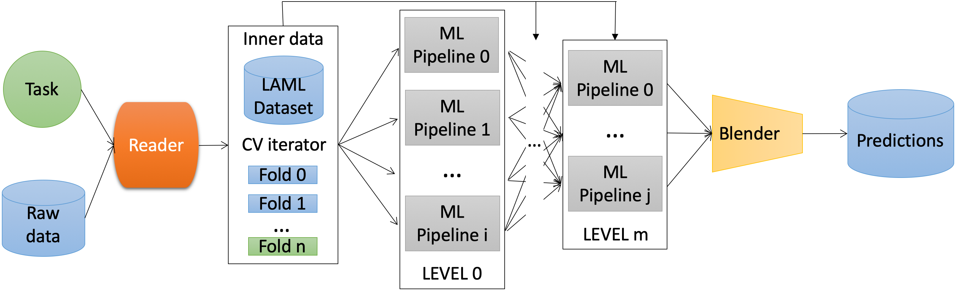
1.3.1 Reader object
First the task and data go into Reader object. It analyzes the data and extracts various valuable information from them. Also it can detect and remove useless features, conduct feature selection, determine types and roles etc. Let’s look at this steps in more detail.
Role and types guessing
Roles can be specified as a string or a specific class object, or defined automatically. For TabularAutoML preset 'numeric', 'datetime' and 'category' roles can be automatically defined. There are two ways of role defining. First is very simple: check if the value can be converted to a date ('datetime'), otherwise check if it can be converted to a number ('numeric'), otherwise declare it a category ('categorical'). But this method may not work well on large data
or when encoding categories with integers. The second method is based on statistics: the distributions of numerical features are considered, and how similar they are to the distributions of real or categorical value. Also different ways of feature encoding (as a number or as a category) are compared and based on normalized Gini index it is decided which encoding is better. For this case a set of specific rules is created, and if at least one of them is fulfilled, then the feature will be
assigned to numerical, otherwise to categorical. This check can be enabled or disabled using the advanced_roles parameter.
If roles are explicitly specified, automatic definition won’t be applied to the specified dataset columns. In the case of specifying a role as an object of a certain class, through its arguments, it is possible to set the processing parameters in more detail.
Feature selection
In general, the AutoML pipeline uses pre-selection, generation and post-selection of features. TabularAutoML has no post-selection stage. There are three feature selection methods: its absence, using features importances and more strict selection (forward selection). The GBM model is used to evaluate features importances. Importances can be calculated in 2 ways: based on splits (how many times a split was made for each feature in the entire ensemble) or using permutation feature importances
(mixing feature values during validation and assessing quality change in this case). Second method is harder but it requires holdout data. Then features with importance above a certain threshold are selected. Faster and more strict feature selection method is forward selection. Features are sorted in descending order of importance, then in blocks (size of 1 by default) a model is built based on selected features, and its quality is measured. Then the next block of features is added, and they are
saved if the quality has improved with them, and so on.
Also LightAutoML can merge some columns if it is adequate and leads to an improvement in the model quality (for example, an intersection between categorical variables). Different columns join options are considered, the best one is chosen by the normalized Gini index.
1.3.2 Machine learning pipelines architecture and training
As a result, after analyzing and processing the data, the Reader object forms and returns a LAMA Dataset. It contains the original data and markup with metainformation. In this dataset it is possible to see the roles defined by the Reader object, selected features etc. Then ML pipelines are trained on this data.
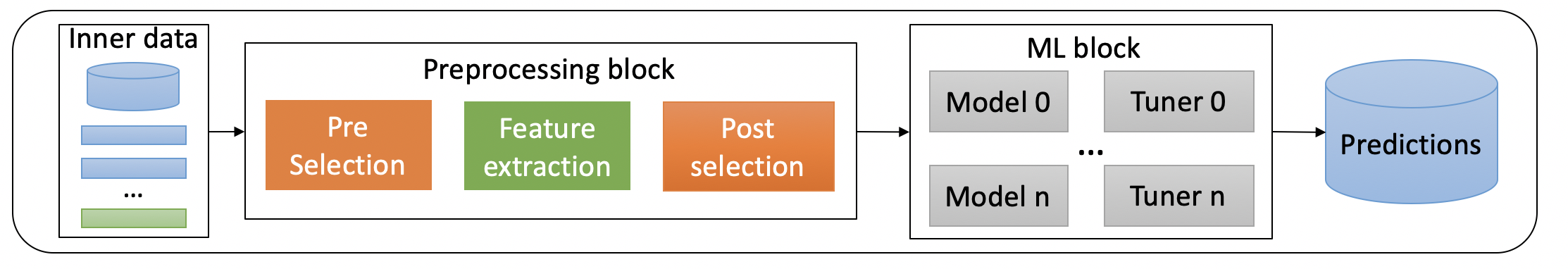
Each such pipeline is one or more machine learning algorithms that share one post-processing block and one validation scheme. Several such pipelines can be trained in parallel on one dataset, and they form a level. Number of levels can be unlimited as possible. List of all levels of AutoML pipeline is available via .levels attribute of AutoML instance. Level predictions can be inputs to other models or ML pipelines (i. e. stacking scheme). As inputs for subsequent levels, it is possible
to use the original data by setting skip_conn argument in True when initializing preset instance. At the last level, if there are several pipelines, blending is used to build a prediction.
Different types of features are processed depending on the models. Numerical features are processed for linear model preprocessing: standardization, replacing missing values with median, discretization, log odds (if feature is probability - output of previous level). Categories are processed using label encoding (by default), one hot encoding, ordinal encoding, frequency encoding, out of fold target encoding.
The following algorithms are available in the LightAutoML: linear regression with L2 regularization, LightGBM, CatBoost, random forest.
By default KFold cross-validation is used during training at all levels (for hyperparameter optimization and building out-of-fold prediction during training), and for each algorithm a separate model is built for each validation fold, and their predictions are averaged. So the predictions at each level and the resulting prediction during training are out-of-fold predictions. But it is also possible to just pass a holdout data for validation or use custom cross-validation schemes, setting
cv_iter iterator returning the indices of the objects for validation. LightAutoML has ready-made iterators, for example, TimeSeriesIterator for time series split. To further reduce the effect of overfitting, it is possible to use nested cross-validation (nested_cv parameter), but it is not used by default.
Prediction on new data is the averaging of models over all folds from validation and blending.
Hyperparameter tuning of machine learning algorithms can be performed during training (early stopping by the number of trees in gradient boosting or the number of training epochs of neural networks etc), based on expert rules (according to data characteristics and empirical recommendations, so-called expert parameters), by the sequential model-based optimization (SMBO, bayesian optimization: Optuna with TPESampler) or by grid search. LightGBM and CatBoost can be used with parameter tuning or with expert parameters, with no tuning. For linear regression parameters are always tuned using warm start model training technique.
At the last level blending is used to build a prediction. There are three available blending methods: choosing the best model based on a given metric (other models are just discarded), simple averaging of all models, or weighted averaging (weights are selected using coordinate descent algorithm with optimization of a given metric). TabularAutoML uses the latter strategy by default. It is worth noting that, unlike stacking, blending can exclude models from composition.
1.3.3 Timing
When creating AutoML object, a certain time limit is set, and it schedules a list of tasks that it can complete during this time, and it will initially allocate approximately equal time for each task. In the process of solving objectives, it understands how to adjust the time allocated to different subtasks. If AutoML finished working earlier than set timeout, it means that it completed the entire list of tasks. If AutoML worked to the limit and turned off, then most likely it sacrificed something, for example, reduced the number of algorithms for training, realized that it would not have time to train the next one, or it might not calculate the full cross-validation cycle for one of the models (then on folds, where the model has not trained, the predictiuons will be NaN, and the model related to this fold will not participate in the final averaging). The resulting quality is evaluated at the blending stage, and if necessary and possible, the composition will be corrected.
If you do not set the time for AutoML during initialization, then by default it will be equal to a very large number, that is, sooner or later AutoML will complete all tasks.
1.3.4 LightAutoML model creation
So the entire AutoML pipeline can be composed from various parts by user (see custom pipeline tutorial), but it is possible to use presets - in a certain sense, fixed strategies for dynamic pipeline building.
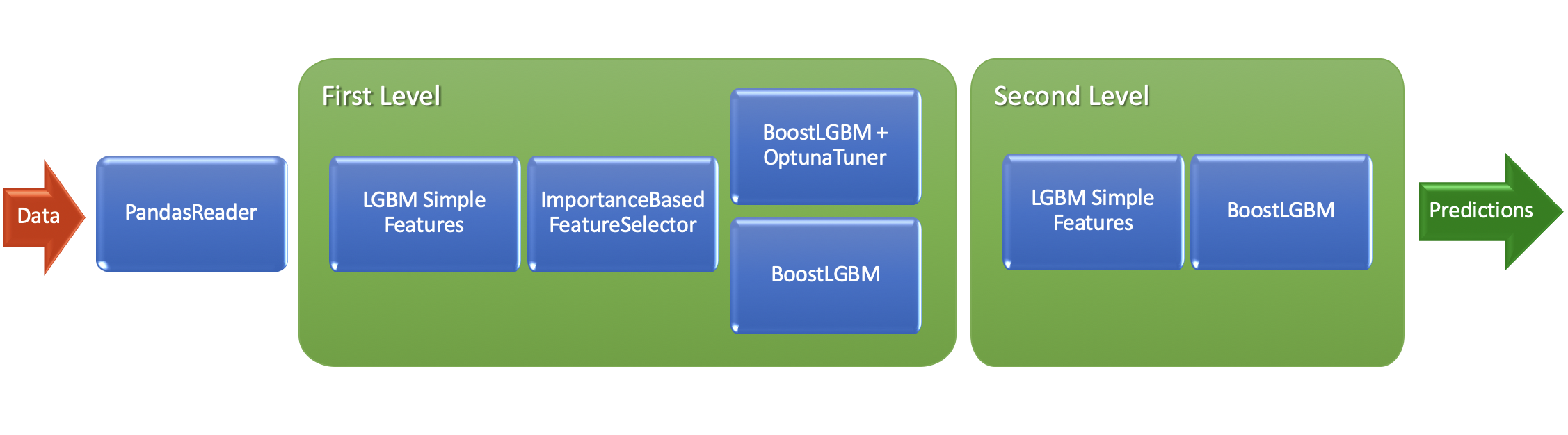
Here is a default AutoML pipeline for binary classification and regression tasks (TabularAutoML preset):

Another example:
Let’s discuss some of the params we can setup: - task - the type of the ML task (the only must have parameter) - timeout - time limit in seconds for model to train - cpu_limit - vCPU count for model to use - reader_params - parameter change for Reader object inside preset, which works on the first step of data preparation: automatic feature typization, preliminary almost-constant features, correct CV setup etc. For example, we setup n_jobs threads for typization algo,
cv folds and random_state as inside CV seed. - general_params - general parameters dictionary, in which it is possible to specify a list of algorithms used ('use_algos'), nested CV using ('nested_cv') etc.
Important note: reader_params key is one of the YAML config keys, which is used inside TabularAutoML preset. More details on its structure with explanation comments can be found on the link attached. Each key from this config can be modified with user settings during preset object initialization. To get more info about different parameters setting (for example, ML algos which can
be used in general_params->use_algos) please take a look at our article on TowardsDataScience.
Moreover, to receive the automatic report for our model we will use ReportDeco decorator and work with the decorated version in the same way as we do with usual one.
[15]:
automl = TabularAutoML(
    task = task,
    timeout = TIMEOUT,
    cpu_limit = N_THREADS,
    reader_params = {'n_jobs': N_THREADS, 'cv': N_FOLDS, 'random_state': RANDOM_STATE},
)
2. AutoML training
To run autoML training use fit_predict method.
Main arguments:
train_data- dataset to train.roles- column roles dict.verbose- controls the verbosity: the higher, the more messages: <1 : messages are not displayed; >=1 : the computation process for layers is displayed; >=2 : the information about folds processing is also displayed; >=3 : the hyperparameters optimization process is also displayed; >=4 : the training process for every algorithm is displayed;
Note: out-of-fold prediction is calculated during training and returned from the fit_predict method
[16]:
%%time
out_of_fold_predictions = automl.fit_predict(train_data, roles = roles, verbose = 1)
[08:50:50] Stdout logging level is INFO.
[08:50:50] Copying TaskTimer may affect the parent PipelineTimer, so copy will create new unlimited TaskTimer
[08:50:50] Task: binary

[08:50:50] Start automl preset with listed constraints:
[08:50:50] - time: 300.00 seconds
[08:50:50] - CPU: 4 cores
[08:50:50] - memory: 16 GB

[08:50:50] Train data shape: (8000, 122)

[08:50:55] Layer 1 train process start. Time left 295.04 secs
[08:50:56] Start fitting Lvl_0_Pipe_0_Mod_0_LinearL2 ...
[08:51:00] Fitting Lvl_0_Pipe_0_Mod_0_LinearL2 finished. score = 0.7351718729105452
[08:51:00] Lvl_0_Pipe_0_Mod_0_LinearL2 fitting and predicting completed
[08:51:00] Time left 290.51 secs

[08:51:02] Selector_LightGBM fitting and predicting completed
[08:51:03] Start fitting Lvl_0_Pipe_1_Mod_0_LightGBM ...
[08:51:15] Fitting Lvl_0_Pipe_1_Mod_0_LightGBM finished. score = 0.7331401653896874
[08:51:15] Lvl_0_Pipe_1_Mod_0_LightGBM fitting and predicting completed
[08:51:15] Start hyperparameters optimization for Lvl_0_Pipe_1_Mod_1_Tuned_LightGBM ... Time budget is 16.51 secs
[08:51:37] Hyperparameters optimization for Lvl_0_Pipe_1_Mod_1_Tuned_LightGBM completed
[08:51:37] Start fitting Lvl_0_Pipe_1_Mod_1_Tuned_LightGBM ...
[08:51:49] Fitting Lvl_0_Pipe_1_Mod_1_Tuned_LightGBM finished. score = 0.7089314555691407
[08:51:49] Lvl_0_Pipe_1_Mod_1_Tuned_LightGBM fitting and predicting completed
[08:51:49] Start fitting Lvl_0_Pipe_1_Mod_2_CatBoost ...
[08:51:54] Fitting Lvl_0_Pipe_1_Mod_2_CatBoost finished. score = 0.7176822653076455
[08:51:54] Lvl_0_Pipe_1_Mod_2_CatBoost fitting and predicting completed
[08:51:54] Start hyperparameters optimization for Lvl_0_Pipe_1_Mod_3_Tuned_CatBoost ... Time budget is 155.49 secs
[08:54:28] Hyperparameters optimization for Lvl_0_Pipe_1_Mod_3_Tuned_CatBoost completed
[08:54:28] Start fitting Lvl_0_Pipe_1_Mod_3_Tuned_CatBoost ...
[08:54:40] Fitting Lvl_0_Pipe_1_Mod_3_Tuned_CatBoost finished. score = 0.7376224015286756
[08:54:40] Lvl_0_Pipe_1_Mod_3_Tuned_CatBoost fitting and predicting completed
[08:54:40] Time left 70.52 secs

[08:54:40] Layer 1 training completed.

[08:54:40] Blending: optimization starts with equal weights and score 0.7485901992886845
[08:54:40] Blending: iteration 0: score = 0.7500463998499898, weights = [0.25878194 0.2476184  0.18001081 0.         0.3135889 ]
[08:54:40] Blending: iteration 1: score = 0.750143026341721, weights = [0.29799867 0.22685595 0.15482728 0.         0.3203181 ]
[08:54:40] Blending: iteration 2: score = 0.7501702390830668, weights = [0.3023924  0.22656146 0.1511439  0.         0.31990227]
[08:54:40] Blending: iteration 3: score = 0.7501702390830668, weights = [0.3023924  0.22656146 0.15114388 0.         0.31990227]
[08:54:40] Blending: no score update. Terminated

[08:54:40] Automl preset training completed in 230.04 seconds

[08:54:40] Model description:
Final prediction for new objects (level 0) =
         0.30239 * (5 averaged models Lvl_0_Pipe_0_Mod_0_LinearL2) +
         0.22656 * (5 averaged models Lvl_0_Pipe_1_Mod_0_LightGBM) +
         0.15114 * (5 averaged models Lvl_0_Pipe_1_Mod_1_Tuned_LightGBM) +
         0.31990 * (5 averaged models Lvl_0_Pipe_1_Mod_3_Tuned_CatBoost)

CPU times: user 13min 39s, sys: 1min 30s, total: 15min 10s
Wall time: 3min 50s
After training we can see logs with all the progress, final scores, weights assigned to the models in the final prediction etc.
Note that in this fit_predict you receive the model with only 3 out of 5 LightGBM models (you can see that from the log line in the end 0.25685 * (3 averaged models Lvl_0_Pipe_1_Mod_0_LightGBM)) - to fix it you can set the bigger timeout to make LightAutoML train all the models.
3. Prediction on holdout and model evaluation
Now we can use trained AutoML model to build predictions on holdout and evaluate model quality. Note that in case of classification tasks LightAutoML model returns probabilities as predictions.
[17]:
%%time

test_predictions = automl.predict(test_data)
print(f'Prediction for test_data:\n{test_predictions}\nShape = {test_predictions.shape}')
Prediction for test_data:
array([[0.06522178],
       [0.06859127],
       [0.0340898 ],
       ...,
       [0.0531715 ],
       [0.04148169],
       [0.18272203]], dtype=float32)
Shape = (2000, 1)
CPU times: user 1.67 s, sys: 90.5 ms, total: 1.76 s
Wall time: 678 ms
[18]:
print(f'OOF score: {roc_auc_score(train_data[TARGET_NAME].values, out_of_fold_predictions.data[:, 0])}')
print(f'HOLDOUT score: {roc_auc_score(test_data[TARGET_NAME].values, test_predictions.data[:, 0])}')
OOF score: 0.7501702390830668
HOLDOUT score: 0.7314741847826086
4. Model analysis
4.1. Reports
You can obtain the description of the resulting pipeline:
[19]:
print(automl.create_model_str_desc())
Final prediction for new objects (level 0) =
         0.30239 * (5 averaged models Lvl_0_Pipe_0_Mod_0_LinearL2) +
         0.22656 * (5 averaged models Lvl_0_Pipe_1_Mod_0_LightGBM) +
         0.15114 * (5 averaged models Lvl_0_Pipe_1_Mod_1_Tuned_LightGBM) +
         0.31990 * (5 averaged models Lvl_0_Pipe_1_Mod_3_Tuned_CatBoost)
Also for this purposes LightAutoML have ReportDeco, use it to build detailed reports:
[20]:
RD = ReportDeco(output_path = 'tabularAutoML_model_report')

automl_rd = RD(
    TabularAutoML(
        task = task,
        timeout = TIMEOUT,
        cpu_limit = N_THREADS,
        reader_params = {'n_jobs': N_THREADS, 'cv': N_FOLDS, 'random_state': RANDOM_STATE}
    )
)
[21]:
%%time
out_of_fold_predictions = automl_rd.fit_predict(train_data, roles = roles, verbose = 1)
[08:54:41] Stdout logging level is INFO.
[08:54:41] Task: binary

[08:54:41] Start automl preset with listed constraints:
[08:54:41] - time: 300.00 seconds
[08:54:41] - CPU: 4 cores
[08:54:41] - memory: 16 GB

[08:54:41] Train data shape: (8000, 122)

[08:54:42] Layer 1 train process start. Time left 298.57 secs
[08:54:43] Start fitting Lvl_0_Pipe_0_Mod_0_LinearL2 ...
[08:54:47] Fitting Lvl_0_Pipe_0_Mod_0_LinearL2 finished. score = 0.7351718729105452
[08:54:47] Lvl_0_Pipe_0_Mod_0_LinearL2 fitting and predicting completed
[08:54:47] Time left 294.28 secs

[08:54:49] Selector_LightGBM fitting and predicting completed
[08:54:50] Start fitting Lvl_0_Pipe_1_Mod_0_LightGBM ...
[08:55:01] Fitting Lvl_0_Pipe_1_Mod_0_LightGBM finished. score = 0.7331401653896874
[08:55:01] Lvl_0_Pipe_1_Mod_0_LightGBM fitting and predicting completed
[08:55:01] Start hyperparameters optimization for Lvl_0_Pipe_1_Mod_1_Tuned_LightGBM ... Time budget is 20.80 secs
[08:55:24] Hyperparameters optimization for Lvl_0_Pipe_1_Mod_1_Tuned_LightGBM completed
[08:55:24] Start fitting Lvl_0_Pipe_1_Mod_1_Tuned_LightGBM ...
[08:55:37] Fitting Lvl_0_Pipe_1_Mod_1_Tuned_LightGBM finished. score = 0.7089314555691407
[08:55:37] Lvl_0_Pipe_1_Mod_1_Tuned_LightGBM fitting and predicting completed
[08:55:37] Start fitting Lvl_0_Pipe_1_Mod_2_CatBoost ...
[08:55:43] Fitting Lvl_0_Pipe_1_Mod_2_CatBoost finished. score = 0.7176822653076455
[08:55:43] Lvl_0_Pipe_1_Mod_2_CatBoost fitting and predicting completed
[08:55:43] Start hyperparameters optimization for Lvl_0_Pipe_1_Mod_3_Tuned_CatBoost ... Time budget is 155.52 secs
[08:58:19] Hyperparameters optimization for Lvl_0_Pipe_1_Mod_3_Tuned_CatBoost completed
[08:58:19] Start fitting Lvl_0_Pipe_1_Mod_3_Tuned_CatBoost ...
[08:58:31] Fitting Lvl_0_Pipe_1_Mod_3_Tuned_CatBoost finished. score = 0.7376224015286756
[08:58:31] Lvl_0_Pipe_1_Mod_3_Tuned_CatBoost fitting and predicting completed
[08:58:31] Time left 69.91 secs

[08:58:31] Layer 1 training completed.

[08:58:31] Blending: optimization starts with equal weights and score 0.7485901992886845
[08:58:31] Blending: iteration 0: score = 0.7500463998499898, weights = [0.25878194 0.2476184  0.18001081 0.         0.3135889 ]
[08:58:31] Blending: iteration 1: score = 0.750143026341721, weights = [0.29799867 0.22685595 0.15482728 0.         0.3203181 ]
[08:58:31] Blending: iteration 2: score = 0.7501702390830668, weights = [0.3023924  0.22656146 0.1511439  0.         0.31990227]
[08:58:32] Blending: iteration 3: score = 0.7501702390830668, weights = [0.3023924  0.22656146 0.15114388 0.         0.31990227]
[08:58:32] Blending: no score update. Terminated

[08:58:32] Automl preset training completed in 230.64 seconds

[08:58:32] Model description:
Final prediction for new objects (level 0) =
         0.30239 * (5 averaged models Lvl_0_Pipe_0_Mod_0_LinearL2) +
         0.22656 * (5 averaged models Lvl_0_Pipe_1_Mod_0_LightGBM) +
         0.15114 * (5 averaged models Lvl_0_Pipe_1_Mod_1_Tuned_LightGBM) +
         0.31990 * (5 averaged models Lvl_0_Pipe_1_Mod_3_Tuned_CatBoost)

CPU times: user 14min 16s, sys: 1min 42s, total: 15min 58s
Wall time: 3min 55s
The report will be available in the folder with specified name (output_path argument in ReportDeco initialization).
[22]:
!ls tabularAutoML_model_report
feature_importance.png            valid_pr_curve.png
lama_interactive_report.html      valid_preds_distribution_by_bins.png
valid_distribution_of_logits.png  valid_roc_curve.png
valid_pie_f1_metric.png
[23]:
%%time

test_predictions = automl_rd.predict(test_data)
print(f'Prediction for test_data:\n{test_predictions}\nShape = {test_predictions.shape}')
Prediction for test_data:
array([[0.06522178],
       [0.06859127],
       [0.0340898 ],
       ...,
       [0.0531715 ],
       [0.04148169],
       [0.18272203]], dtype=float32)
Shape = (2000, 1)
CPU times: user 14.1 s, sys: 11.2 s, total: 25.3 s
Wall time: 3.71 s
[24]:
print(f'OOF score: {roc_auc_score(train_data[TARGET_NAME].values, out_of_fold_predictions.data[:, 0])}')
print(f'HOLDOUT score: {roc_auc_score(test_data[TARGET_NAME].values, test_predictions.data[:, 0])}')
OOF score: 0.7501702390830668
HOLDOUT score: 0.7314741847826086
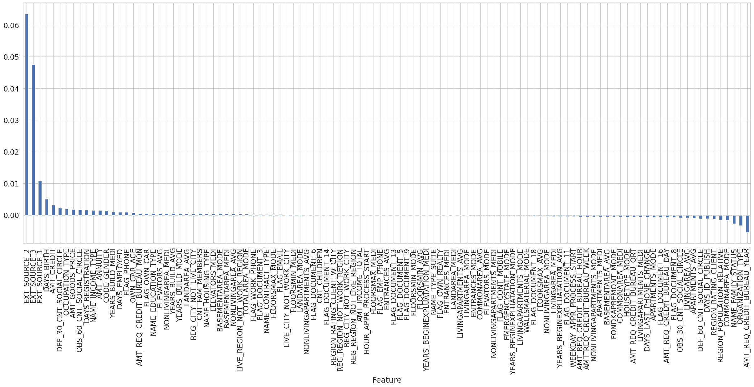
4.2 Feature importances calculation
For feature importances calculation we have 2 different methods in LightAutoML: - Fast (fast) - this method uses feature importances from feature selector LGBM model inside LightAutoML. It works extremely fast and almost always (almost because of situations, when feature selection is turned off or selector was removed from the final models with all GBM models). There is no need to use new labelled data. - Accurate (accurate) - this method calculate features permutation importances for
the whole LightAutoML model based on the new labelled data. It always works but can take a lot of time to finish (depending on the model structure, new labelled dataset size etc.).
In the cell below we will use automl_rd.model instead automl_rd because we want to take the importances from the model, not from the report. But be careful - everything, which is calculated using automl_rd.model will not go to the report.
[25]:
%%time
# Fast feature importances calculation
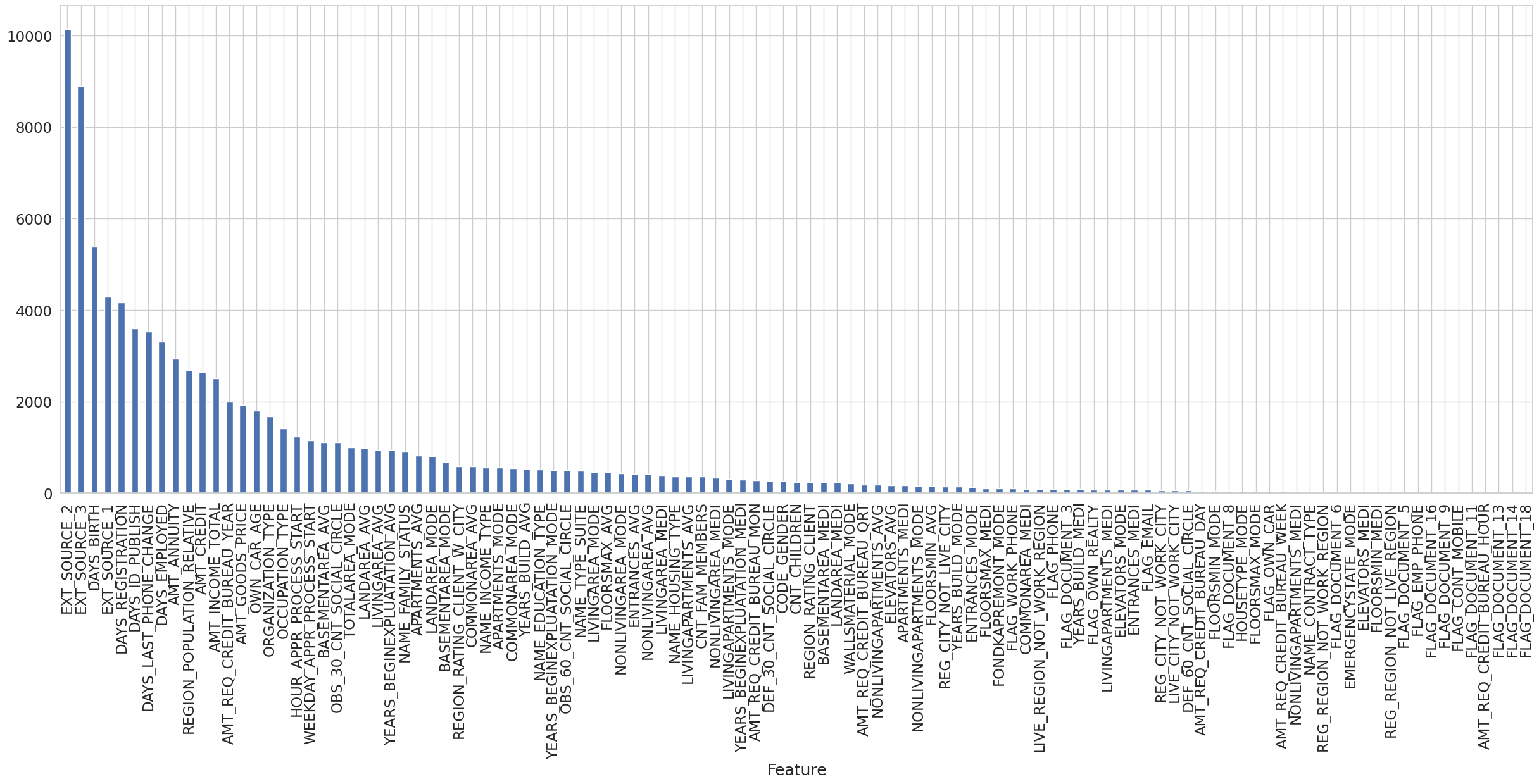
fast_fi = automl_rd.model.get_feature_scores('fast')
fast_fi.set_index('Feature')['Importance'].plot.bar(figsize = (30, 10), grid = True)
CPU times: user 397 ms, sys: 120 ms, total: 517 ms
Wall time: 284 ms
[25]:
<Axes: xlabel='Feature'>

[26]:
%%time

# Accurate feature importances calculation with detailed info (Permutation importances) -  can take long time to calculate
accurate_fi = automl_rd.model.get_feature_scores('accurate', test_data, silent = True)
CPU times: user 3min 18s, sys: 15.8 s, total: 3min 33s
Wall time: 1min 14s
[27]:
accurate_fi.set_index('Feature')['Importance'].plot.bar(figsize = (30, 10), grid = True)
[27]:
<Axes: xlabel='Feature'>

4.3 Shapley values
[28]:
explainer = SSWARM(automl_rd.model)
shap_values = explainer.shap_values(test_data, n_jobs=N_THREADS)
100%|████████████████████████████████████████████████████████████████████████████████████████████| 3000/3000 [03:42<00:00, 13.46it/s]
[29]:
# summary plot

# !pip install shap
import shap
shap.summary_plot(shap_values[1], test_data[explainer.used_feats])

[30]:
# dependence plots
import matplotlib.pyplot as plt

feats = ["EXT_SOURCE_2", "EXT_SOURCE_3", "DAYS_BIRTH", "DAYS_REGISTRATION", "REGION_RATING_CLIENT_W_CITY"]
fig, ax = plt.subplots(nrows=len(feats), ncols=1, figsize=(10, 5*len(feats)))

for i, feat in enumerate(feats):
    shap.dependence_plot(feat, shap_values[1], test_data[explainer.used_feats],
                         show=False, ax=ax[i], interaction_index="EXT_SOURCE_1")

[42]:
# individual force plot
shap.force_plot(explainer.expected_value[1], shap_values[1][0], test_data[explainer.used_feats].iloc[0], matplotlib=True)

[43]:
# overall force plot
shap.initjs()
shap.force_plot(explainer.expected_value[1], shap_values[1][:500], test_data[explainer.used_feats].iloc[:500])

[43]:
Have you run `initjs()` in this notebook? If this notebook was from another user you must also trust this notebook (File -> Trust notebook). If you are viewing this notebook on github the Javascript has been stripped for security. If you are using JupyterLab this error is because a JupyterLab extension has not yet been written.
Bonus: where is the automatic report?
As we used automl_rd in our training and prediction cells, it is already ready in the folder we specified - you can check the output folder and find the tabularAutoML_model_report folder with lama_interactive_report.html report inside (or just click this link for short). It’s interactive so you can click the black triangles on the left of the texts to go deeper in selected part.
5. Spending more from TIMEOUT - TabularUtilizedAutoML usage
To spend (almost) all the TIMEOUT time for building the model we can use TabularUtilizedAutoML preset instead of TabularAutoML, which has the same API. By default TabularUtilizedAutoML model trains with 7 different parameter configurations (see this for more details) sequentially, and if there is time left, then whole AutoML pipeline with these configs is run again with another
cross-validation seed, and so on. Then results for each pipeline model are averaged over the considered validation seeds, and all averaged results at the end are also combined through blending. User can set his own set of configs by passing list of paths to according files in configs_list argument during TabularUtilizedAutoML instance initialization. Such configs allow the user to configure all pipeline parameters and can be used for any available preset.
[44]:
utilized_automl = TabularUtilizedAutoML(
    task = task,
    timeout = 900,
    cpu_limit = N_THREADS,
    reader_params = {'n_jobs': N_THREADS, 'cv': N_FOLDS, 'random_state': RANDOM_STATE},
)
[45]:
%%time

out_of_fold_predictions = utilized_automl.fit_predict(train_data, roles = roles, verbose = 1)
[09:05:31] Start automl utilizator with listed constraints:
[09:05:31] - time: 900.00 seconds
[09:05:31] - CPU: 4 cores
[09:05:31] - memory: 16 GB

[09:05:31] If one preset completes earlier, next preset configuration will be started

[09:05:31] ==================================================
[09:05:31] Start 0 automl preset configuration:
[09:05:31] conf_0_sel_type_0.yml, random state: {'reader_params': {'random_state': 42}, 'nn_params': {'random_state': 42}, 'general_params': {'return_all_predictions': False}}
[09:05:31] Stdout logging level is INFO.
[09:05:31] Task: binary

[09:05:31] Start automl preset with listed constraints:
[09:05:31] - time: 900.00 seconds
[09:05:31] - CPU: 4 cores
[09:05:31] - memory: 16 GB

[09:05:31] Train data shape: (8000, 122)

[09:05:37] Layer 1 train process start. Time left 894.60 secs
[09:05:38] Start fitting Lvl_0_Pipe_0_Mod_0_LinearL2 ...
[09:05:42] Fitting Lvl_0_Pipe_0_Mod_0_LinearL2 finished. score = 0.7351718729105452
[09:05:42] Lvl_0_Pipe_0_Mod_0_LinearL2 fitting and predicting completed
[09:05:42] Time left 889.74 secs

[09:05:43] Start fitting Lvl_0_Pipe_1_Mod_0_LightGBM ...
[09:06:01] Fitting Lvl_0_Pipe_1_Mod_0_LightGBM finished. score = 0.7208359669101568
[09:06:01] Lvl_0_Pipe_1_Mod_0_LightGBM fitting and predicting completed
[09:06:01] Start hyperparameters optimization for Lvl_0_Pipe_1_Mod_1_Tuned_LightGBM ... Time budget is 92.70 secs
[09:07:35] Hyperparameters optimization for Lvl_0_Pipe_1_Mod_1_Tuned_LightGBM completed
[09:07:35] Start fitting Lvl_0_Pipe_1_Mod_1_Tuned_LightGBM ...
[09:07:39] Fitting Lvl_0_Pipe_1_Mod_1_Tuned_LightGBM finished. score = 0.7387079347889174
[09:07:39] Lvl_0_Pipe_1_Mod_1_Tuned_LightGBM fitting and predicting completed
[09:07:40] Start fitting Lvl_0_Pipe_1_Mod_2_CatBoost ...
[09:07:46] Fitting Lvl_0_Pipe_1_Mod_2_CatBoost finished. score = 0.7216183332238446
[09:07:46] Lvl_0_Pipe_1_Mod_2_CatBoost fitting and predicting completed
[09:07:46] Start hyperparameters optimization for Lvl_0_Pipe_1_Mod_3_Tuned_CatBoost ... Time budget is 300.00 secs
[09:10:12] Hyperparameters optimization for Lvl_0_Pipe_1_Mod_3_Tuned_CatBoost completed
[09:10:12] Start fitting Lvl_0_Pipe_1_Mod_3_Tuned_CatBoost ...
[09:10:18] Fitting Lvl_0_Pipe_1_Mod_3_Tuned_CatBoost finished. score = 0.7400775010369544
[09:10:18] Lvl_0_Pipe_1_Mod_3_Tuned_CatBoost fitting and predicting completed
[09:10:18] Time left 613.68 secs

[09:10:18] Layer 1 training completed.

[09:10:18] Blending: optimization starts with equal weights and score 0.7511137558494106
[09:10:18] Blending: iteration 0: score = 0.7520976665286894, weights = [0.24006502 0.11192521 0.24787743 0.09496131 0.305171  ]
[09:10:18] Blending: iteration 1: score = 0.7521652731829703, weights = [0.24298649 0.07254668 0.27720243 0.08237854 0.32488596]
[09:10:18] Blending: iteration 2: score = 0.7521720763683065, weights = [0.25121042 0.07175855 0.274191   0.0814836  0.32135648]
[09:10:18] Blending: iteration 3: score = 0.7521720763683065, weights = [0.25121042 0.07175854 0.274191   0.08148359 0.32135645]
[09:10:18] Blending: no score update. Terminated

[09:10:18] Automl preset training completed in 286.84 seconds

[09:10:18] Model description:
Final prediction for new objects (level 0) =
         0.25121 * (5 averaged models Lvl_0_Pipe_0_Mod_0_LinearL2) +
         0.07176 * (5 averaged models Lvl_0_Pipe_1_Mod_0_LightGBM) +
         0.27419 * (5 averaged models Lvl_0_Pipe_1_Mod_1_Tuned_LightGBM) +
         0.08148 * (5 averaged models Lvl_0_Pipe_1_Mod_2_CatBoost) +
         0.32136 * (5 averaged models Lvl_0_Pipe_1_Mod_3_Tuned_CatBoost)

[09:10:18] ==================================================
[09:10:18] Start 1 automl preset configuration:
[09:10:18] conf_1_sel_type_1.yml, random state: {'reader_params': {'random_state': 43}, 'nn_params': {'random_state': 43}, 'general_params': {'return_all_predictions': False}}
[09:10:18] Stdout logging level is INFO.
[09:10:18] Task: binary

[09:10:18] Start automl preset with listed constraints:
[09:10:18] - time: 613.07 seconds
[09:10:18] - CPU: 4 cores
[09:10:18] - memory: 16 GB

[09:10:18] Train data shape: (8000, 122)

[09:10:20] Layer 1 train process start. Time left 611.60 secs
[09:10:21] Start fitting Lvl_0_Pipe_0_Mod_0_LinearL2 ...
[09:10:25] Fitting Lvl_0_Pipe_0_Mod_0_LinearL2 finished. score = 0.7343900380957119
[09:10:25] Lvl_0_Pipe_0_Mod_0_LinearL2 fitting and predicting completed
[09:10:25] Time left 606.69 secs

[09:10:28] Selector_LightGBM fitting and predicting completed
[09:10:29] Start fitting Lvl_0_Pipe_1_Mod_0_LightGBM ...
[09:10:49] Fitting Lvl_0_Pipe_1_Mod_0_LightGBM finished. score = 0.7440739472230141
[09:10:49] Lvl_0_Pipe_1_Mod_0_LightGBM fitting and predicting completed
[09:10:49] Start hyperparameters optimization for Lvl_0_Pipe_1_Mod_1_Tuned_LightGBM ... Time budget is 38.55 secs
[09:11:32] Hyperparameters optimization for Lvl_0_Pipe_1_Mod_1_Tuned_LightGBM completed
[09:11:32] Start fitting Lvl_0_Pipe_1_Mod_1_Tuned_LightGBM ...
[09:11:49] Fitting Lvl_0_Pipe_1_Mod_1_Tuned_LightGBM finished. score = 0.7309214765718494
[09:11:49] Lvl_0_Pipe_1_Mod_1_Tuned_LightGBM fitting and predicting completed
[09:11:49] Start fitting Lvl_0_Pipe_1_Mod_2_CatBoost ...
[09:11:53] Fitting Lvl_0_Pipe_1_Mod_2_CatBoost finished. score = 0.7073296243217277
[09:11:53] Lvl_0_Pipe_1_Mod_2_CatBoost fitting and predicting completed
[09:11:53] Start hyperparameters optimization for Lvl_0_Pipe_1_Mod_3_Tuned_CatBoost ... Time budget is 300.00 secs
[09:14:42] Hyperparameters optimization for Lvl_0_Pipe_1_Mod_3_Tuned_CatBoost completed
[09:14:42] Start fitting Lvl_0_Pipe_1_Mod_3_Tuned_CatBoost ...
[09:14:51] Fitting Lvl_0_Pipe_1_Mod_3_Tuned_CatBoost finished. score = 0.7434170146389666
[09:14:51] Lvl_0_Pipe_1_Mod_3_Tuned_CatBoost fitting and predicting completed
[09:14:51] Time left 340.03 secs

[09:14:51] Layer 1 training completed.

[09:14:51] Blending: optimization starts with equal weights and score 0.751036369616209
[09:14:52] Blending: iteration 0: score = 0.7539285737823521, weights = [0.10462688 0.3023047  0.40002117 0.05180185 0.14124545]
[09:14:52] Blending: iteration 1: score = 0.7542955205914349, weights = [0.1847324  0.21803026 0.4247732  0.         0.17246413]
[09:14:52] Blending: iteration 2: score = 0.754351009071835, weights = [0.16244903 0.24964364 0.41634628 0.         0.171561  ]
[09:14:52] Blending: iteration 3: score = 0.754351009071835, weights = [0.16244903 0.24964364 0.41634628 0.         0.171561  ]
[09:14:52] Blending: no score update. Terminated

[09:14:52] Automl preset training completed in 273.55 seconds

[09:14:52] Model description:
Final prediction for new objects (level 0) =
         0.16245 * (5 averaged models Lvl_0_Pipe_0_Mod_0_LinearL2) +
         0.24964 * (5 averaged models Lvl_0_Pipe_1_Mod_0_LightGBM) +
         0.41635 * (5 averaged models Lvl_0_Pipe_1_Mod_1_Tuned_LightGBM) +
         0.17156 * (5 averaged models Lvl_0_Pipe_1_Mod_3_Tuned_CatBoost)

[09:14:52] ==================================================
[09:14:52] Start 2 automl preset configuration:
[09:14:52] conf_2_select_mode_1_no_typ.yml, random state: {'reader_params': {'random_state': 44}, 'nn_params': {'random_state': 44}, 'general_params': {'return_all_predictions': False}}
[09:14:52] Stdout logging level is INFO.
[09:14:52] Task: binary

[09:14:52] Start automl preset with listed constraints:
[09:14:52] - time: 339.45 seconds
[09:14:52] - CPU: 4 cores
[09:14:52] - memory: 16 GB

[09:14:52] Train data shape: (8000, 122)

[09:14:52] Layer 1 train process start. Time left 339.28 secs
[09:14:53] Start fitting Lvl_0_Pipe_0_Mod_0_LinearL2 ...
[09:14:58] Fitting Lvl_0_Pipe_0_Mod_0_LinearL2 finished. score = 0.7370140479399211
[09:14:58] Lvl_0_Pipe_0_Mod_0_LinearL2 fitting and predicting completed
[09:14:58] Time left 333.87 secs

[09:15:01] Selector_LightGBM fitting and predicting completed
[09:15:02] Start fitting Lvl_0_Pipe_1_Mod_0_LightGBM ...
[09:15:20] Fitting Lvl_0_Pipe_1_Mod_0_LightGBM finished. score = 0.7306162899296487
[09:15:20] Lvl_0_Pipe_1_Mod_0_LightGBM fitting and predicting completed
[09:15:20] Start hyperparameters optimization for Lvl_0_Pipe_1_Mod_1_Tuned_LightGBM ... Time budget is 1.00 secs
[09:15:33] Hyperparameters optimization for Lvl_0_Pipe_1_Mod_1_Tuned_LightGBM completed
[09:15:33] Start fitting Lvl_0_Pipe_1_Mod_1_Tuned_LightGBM ...
[09:15:50] Fitting Lvl_0_Pipe_1_Mod_1_Tuned_LightGBM finished. score = 0.7192733602781992
[09:15:50] Lvl_0_Pipe_1_Mod_1_Tuned_LightGBM fitting and predicting completed
[09:15:51] Start fitting Lvl_0_Pipe_1_Mod_2_CatBoost ...
[09:15:57] Fitting Lvl_0_Pipe_1_Mod_2_CatBoost finished. score = 0.7293459013678443
[09:15:57] Lvl_0_Pipe_1_Mod_2_CatBoost fitting and predicting completed
[09:15:57] Start hyperparameters optimization for Lvl_0_Pipe_1_Mod_3_Tuned_CatBoost ... Time budget is 179.94 secs
[09:18:45] Hyperparameters optimization for Lvl_0_Pipe_1_Mod_3_Tuned_CatBoost completed
[09:18:45] Start fitting Lvl_0_Pipe_1_Mod_3_Tuned_CatBoost ...
[09:18:54] Fitting Lvl_0_Pipe_1_Mod_3_Tuned_CatBoost finished. score = 0.7519280120943626
[09:18:54] Lvl_0_Pipe_1_Mod_3_Tuned_CatBoost fitting and predicting completed
[09:18:54] Time left 97.01 secs

[09:18:54] Layer 1 training completed.

[09:18:54] Blending: optimization starts with equal weights and score 0.7553933846250989
[09:18:55] Blending: iteration 0: score = 0.7573044419060059, weights = [0.18904768 0.10002336 0.42633003 0.         0.28459892]
[09:18:55] Blending: iteration 1: score = 0.7573339932423109, weights = [0.19110394 0.09505802 0.4097812  0.         0.3040569 ]
[09:18:55] Blending: iteration 2: score = 0.7573339932423109, weights = [0.19110394 0.09505802 0.40978116 0.         0.3040569 ]
[09:18:55] Blending: no score update. Terminated

[09:18:55] Automl preset training completed in 242.82 seconds

[09:18:55] Model description:
Final prediction for new objects (level 0) =
         0.19110 * (5 averaged models Lvl_0_Pipe_0_Mod_0_LinearL2) +
         0.09506 * (5 averaged models Lvl_0_Pipe_1_Mod_0_LightGBM) +
         0.40978 * (5 averaged models Lvl_0_Pipe_1_Mod_1_Tuned_LightGBM) +
         0.30406 * (5 averaged models Lvl_0_Pipe_1_Mod_3_Tuned_CatBoost)

[09:18:55] ==================================================
[09:18:55] Blending: optimization starts with equal weights and score 0.7599013453086403
[09:18:55] Blending: iteration 0: score = 0.7607196409448859, weights = [0.10080308 0.3555537  0.5436432 ]
[09:18:55] Blending: iteration 1: score = 0.7607196409448859, weights = [0.10080308 0.3555537  0.5436432 ]
[09:18:55] Blending: no score update. Terminated

CPU times: user 48min 10s, sys: 4min 52s, total: 53min 2s
Wall time: 13min 23s
[46]:
print('out_of_fold_predictions:\n{}\nShape = {}'.format(out_of_fold_predictions, out_of_fold_predictions.shape))
out_of_fold_predictions:
array([[0.02990189],
       [0.01378681],
       [0.02714774],
       ...,
       [0.02049532],
       [0.13665317],
       [0.07793609]], dtype=float32)
Shape = (8000, 1)
[47]:
print(utilized_automl.create_model_str_desc())
Final prediction for new objects =
        0.10080 * 1 averaged models with config = "conf_0_sel_type_0.yml" and different CV random_states. Their structures:

            Model #0.
                ================================================================================
                Final prediction for new objects (level 0) =
                         0.25121 * (5 averaged models Lvl_0_Pipe_0_Mod_0_LinearL2) +
                         0.07176 * (5 averaged models Lvl_0_Pipe_1_Mod_0_LightGBM) +
                         0.27419 * (5 averaged models Lvl_0_Pipe_1_Mod_1_Tuned_LightGBM) +
                         0.08148 * (5 averaged models Lvl_0_Pipe_1_Mod_2_CatBoost) +
                         0.32136 * (5 averaged models Lvl_0_Pipe_1_Mod_3_Tuned_CatBoost)
                ================================================================================


        + 0.35555 * 1 averaged models with config = "conf_1_sel_type_1.yml" and different CV random_states. Their structures:

            Model #0.
                ================================================================================
                Final prediction for new objects (level 0) =
                         0.16245 * (5 averaged models Lvl_0_Pipe_0_Mod_0_LinearL2) +
                         0.24964 * (5 averaged models Lvl_0_Pipe_1_Mod_0_LightGBM) +
                         0.41635 * (5 averaged models Lvl_0_Pipe_1_Mod_1_Tuned_LightGBM) +
                         0.17156 * (5 averaged models Lvl_0_Pipe_1_Mod_3_Tuned_CatBoost)
                ================================================================================


        + 0.54364 * 1 averaged models with config = "conf_2_select_mode_1_no_typ.yml" and different CV random_states. Their structures:

            Model #0.
                ================================================================================
                Final prediction for new objects (level 0) =
                         0.19110 * (5 averaged models Lvl_0_Pipe_0_Mod_0_LinearL2) +
                         0.09506 * (5 averaged models Lvl_0_Pipe_1_Mod_0_LightGBM) +
                         0.40978 * (5 averaged models Lvl_0_Pipe_1_Mod_1_Tuned_LightGBM) +
                         0.30406 * (5 averaged models Lvl_0_Pipe_1_Mod_3_Tuned_CatBoost)
                ================================================================================
Feature importances calculation for TabularUtilizedAutoML:
[48]:
%%time

# Fast feature importances calculation
fast_fi = utilized_automl.get_feature_scores('fast', silent=False)
fast_fi.set_index('Feature')['Importance'].plot.bar(figsize = (30, 10), grid = True)
CPU times: user 4.27 s, sys: 3.49 s, total: 7.77 s
Wall time: 690 ms
[48]:
<Axes: xlabel='Feature'>
Note that in TabularUtilizedAutoML the first config doesn’t have a LGBM feature selector (but second one already has it), so if there is enough time only for training with the first config, then 'fast' feature importance calculation method won’t work. 'accurate' method will still work correctly.
[49]:
%%time

# Accurate feature importances calculation
fast_fi = utilized_automl.get_feature_scores('accurate', test_data, silent=True)
fast_fi.set_index('Feature')['Importance'].plot.bar(figsize = (30, 10), grid = True)
CPU times: user 13min 54s, sys: 1min 6s, total: 15min
Wall time: 4min 36s
[49]:
<Axes: xlabel='Feature'>
Prediction on holdout and metric calculation:
[50]:
%%time

test_predictions = utilized_automl.predict(test_data)
print(f'Prediction for test_data:\n{test_predictions}\nShape = {test_predictions.shape}')
Prediction for test_data:
array([[0.04470912],
       [0.05975739],
       [0.01950551],
       ...,
       [0.03931152],
       [0.02568556],
       [0.18183662]], dtype=float32)
Shape = (2000, 1)
CPU times: user 7.15 s, sys: 149 ms, total: 7.3 s
Wall time: 2.53 s
[51]:
print(f'OOF score: {roc_auc_score(train_data[TARGET_NAME].values, out_of_fold_predictions.data[:, 0])}')
print(f'HOLDOUT score: {roc_auc_score(test_data[TARGET_NAME].values, test_predictions.data[:, 0])}')
OOF score: 0.7607196409448859
HOLDOUT score: 0.7316508152173913
5.1 Report
[13]:
RDU = ReportDecoUtilized(output_path = 'tabularUtilizedAutoML_model_report')

automl_rdu = RDU(
    TabularUtilizedAutoML(
        task = task,
        timeout = 900,
        cpu_limit = N_THREADS,
        reader_params = {'n_jobs': N_THREADS, 'cv': N_FOLDS, 'random_state': RANDOM_STATE},
    )
)
[14]:
%%time
out_of_fold_predictions = automl_rdu.fit_predict(train_data, roles = roles, verbose = 1)
[10:00:44] Start automl utilizator with listed constraints:
[10:00:44] - time: 900.00 seconds
[10:00:44] - CPU: 4 cores
[10:00:44] - memory: 16 GB

[10:00:44] If one preset completes earlier, next preset configuration will be started

[10:00:44] ==================================================
[10:00:44] Start 0 automl preset configuration:
[10:00:44] conf_0_sel_type_0.yml, random state: {'reader_params': {'random_state': 42}, 'nn_params': {'random_state': 42}, 'general_params': {'return_all_predictions': False}}
[10:00:44] Stdout logging level is INFO.
[10:00:44] Task: binary

[10:00:44] Start automl preset with listed constraints:
[10:00:44] - time: 900.00 seconds
[10:00:44] - CPU: 4 cores
[10:00:44] - memory: 16 GB

[10:00:44] Train data shape: (8000, 122)

[10:00:46] Layer 1 train process start. Time left 897.88 secs
[10:00:46] Start fitting Lvl_0_Pipe_0_Mod_0_LinearL2 ...
[10:00:47] Fitting Lvl_0_Pipe_0_Mod_0_LinearL2 finished. score = 0.735187286377323
[10:00:47] Lvl_0_Pipe_0_Mod_0_LinearL2 fitting and predicting completed
[10:00:47] Time left 896.30 secs

[10:00:48] Start fitting Lvl_0_Pipe_1_Mod_0_LightGBM ...
[10:00:57] Fitting Lvl_0_Pipe_1_Mod_0_LightGBM finished. score = 0.7208359669101568
[10:00:57] Lvl_0_Pipe_1_Mod_0_LightGBM fitting and predicting completed
[10:00:57] Start hyperparameters optimization for Lvl_0_Pipe_1_Mod_1_Tuned_LightGBM ... Time budget is 154.80 secs
[10:00:57] Copying TaskTimer may affect the parent PipelineTimer, so copy will create new unlimited TaskTimer
[10:03:33] Hyperparameters optimization for Lvl_0_Pipe_1_Mod_1_Tuned_LightGBM completed
[10:03:33] Start fitting Lvl_0_Pipe_1_Mod_1_Tuned_LightGBM ...
[10:03:38] Fitting Lvl_0_Pipe_1_Mod_1_Tuned_LightGBM finished. score = 0.6872182391698073
[10:03:38] Lvl_0_Pipe_1_Mod_1_Tuned_LightGBM fitting and predicting completed
[10:03:38] Start fitting Lvl_0_Pipe_1_Mod_2_CatBoost ...
[10:03:44] Fitting Lvl_0_Pipe_1_Mod_2_CatBoost finished. score = 0.7203027672594154
[10:03:44] Lvl_0_Pipe_1_Mod_2_CatBoost fitting and predicting completed
[10:03:44] Start hyperparameters optimization for Lvl_0_Pipe_1_Mod_3_Tuned_CatBoost ... Time budget is 300.00 secs
[10:05:50] Hyperparameters optimization for Lvl_0_Pipe_1_Mod_3_Tuned_CatBoost completed
[10:05:50] Start fitting Lvl_0_Pipe_1_Mod_3_Tuned_CatBoost ...
[10:05:58] Fitting Lvl_0_Pipe_1_Mod_3_Tuned_CatBoost finished. score = 0.7436991342308862
[10:05:58] Lvl_0_Pipe_1_Mod_3_Tuned_CatBoost fitting and predicting completed
[10:05:58] Time left 585.48 secs

[10:05:58] Layer 1 training completed.

[10:05:58] Blending: optimization starts with equal weights and score 0.7474317443856182
[10:05:58] Blending: iteration 0: score = 0.7499482851614662, weights = [0.28868666 0.19095857 0.06477723 0.08807771 0.36749983]
[10:05:58] Blending: iteration 1: score = 0.7499771986991458, weights = [0.3108266  0.17629829 0.05980414 0.0813158  0.37175515]
[10:05:58] Blending: iteration 2: score = 0.749987934976005, weights = [0.30671465 0.1773502  0.06016096 0.08180097 0.37397328]
[10:05:58] Blending: iteration 3: score = 0.749987934976005, weights = [0.30671465 0.1773502  0.06016096 0.08180097 0.37397328]
[10:05:58] Blending: no score update. Terminated

[10:05:58] Automl preset training completed in 314.89 seconds

[10:05:58] Model description:
Final prediction for new objects (level 0) =
         0.30671 * (5 averaged models Lvl_0_Pipe_0_Mod_0_LinearL2) +
         0.17735 * (5 averaged models Lvl_0_Pipe_1_Mod_0_LightGBM) +
         0.06016 * (5 averaged models Lvl_0_Pipe_1_Mod_1_Tuned_LightGBM) +
         0.08180 * (5 averaged models Lvl_0_Pipe_1_Mod_2_CatBoost) +
         0.37397 * (5 averaged models Lvl_0_Pipe_1_Mod_3_Tuned_CatBoost)

[10:05:58] ==================================================
[10:05:58] Start 1 automl preset configuration:
[10:05:58] conf_1_sel_type_1.yml, random state: {'reader_params': {'random_state': 43}, 'nn_params': {'random_state': 43}, 'general_params': {'return_all_predictions': False}}
[10:05:59] Stdout logging level is INFO.
[10:05:59] Task: binary

[10:05:59] Start automl preset with listed constraints:
[10:05:59] - time: 585.08 seconds
[10:05:59] - CPU: 4 cores
[10:05:59] - memory: 16 GB

[10:05:59] Train data shape: (8000, 122)

[10:06:01] Layer 1 train process start. Time left 582.60 secs
[10:06:01] Start fitting Lvl_0_Pipe_0_Mod_0_LinearL2 ...
[10:06:04] Fitting Lvl_0_Pipe_0_Mod_0_LinearL2 finished. score = 0.7343764317250391
[10:06:04] Lvl_0_Pipe_0_Mod_0_LinearL2 fitting and predicting completed
[10:06:04] Time left 579.34 secs

[10:06:07] Selector_LightGBM fitting and predicting completed
[10:06:08] Start fitting Lvl_0_Pipe_1_Mod_0_LightGBM ...
[10:06:27] Fitting Lvl_0_Pipe_1_Mod_0_LightGBM finished. score = 0.7440739472230141
[10:06:27] Lvl_0_Pipe_1_Mod_0_LightGBM fitting and predicting completed
[10:06:27] Start hyperparameters optimization for Lvl_0_Pipe_1_Mod_1_Tuned_LightGBM ... Time budget is 35.96 secs
[10:07:05] Hyperparameters optimization for Lvl_0_Pipe_1_Mod_1_Tuned_LightGBM completed
[10:07:05] Start fitting Lvl_0_Pipe_1_Mod_1_Tuned_LightGBM ...
[10:07:31] Fitting Lvl_0_Pipe_1_Mod_1_Tuned_LightGBM finished. score = 0.7309214765718494
[10:07:31] Lvl_0_Pipe_1_Mod_1_Tuned_LightGBM fitting and predicting completed
[10:07:31] Start fitting Lvl_0_Pipe_1_Mod_2_CatBoost ...
[10:07:35] Fitting Lvl_0_Pipe_1_Mod_2_CatBoost finished. score = 0.7081926721615145
[10:07:35] Lvl_0_Pipe_1_Mod_2_CatBoost fitting and predicting completed
[10:07:35] Start hyperparameters optimization for Lvl_0_Pipe_1_Mod_3_Tuned_CatBoost ... Time budget is 300.00 secs
[10:10:49] Hyperparameters optimization for Lvl_0_Pipe_1_Mod_3_Tuned_CatBoost completed
[10:10:49] Start fitting Lvl_0_Pipe_1_Mod_3_Tuned_CatBoost ...
[10:10:57] Fitting Lvl_0_Pipe_1_Mod_3_Tuned_CatBoost finished. score = 0.7361510001001345
[10:10:57] Lvl_0_Pipe_1_Mod_3_Tuned_CatBoost fitting and predicting completed
[10:10:57] Time left 286.73 secs

[10:10:57] Layer 1 training completed.

[10:10:57] Blending: optimization starts with equal weights and score 0.7497769299308051
[10:10:57] Blending: iteration 0: score = 0.7534326853511901, weights = [0.08608949 0.3215845  0.44514042 0.05545893 0.09172665]
[10:10:57] Blending: iteration 1: score = 0.7539372903635644, weights = [0.14486776 0.31182623 0.40830123 0.05086922 0.08413548]
[10:10:57] Blending: iteration 2: score = 0.7539333572720418, weights = [0.14514707 0.3117244  0.4081679  0.05085261 0.08410801]
[10:10:57] Blending: no score update. Terminated

[10:10:57] Automl preset training completed in 298.63 seconds

[10:10:57] Model description:
Final prediction for new objects (level 0) =
         0.14487 * (5 averaged models Lvl_0_Pipe_0_Mod_0_LinearL2) +
         0.31183 * (5 averaged models Lvl_0_Pipe_1_Mod_0_LightGBM) +
         0.40830 * (5 averaged models Lvl_0_Pipe_1_Mod_1_Tuned_LightGBM) +
         0.05087 * (5 averaged models Lvl_0_Pipe_1_Mod_2_CatBoost) +
         0.08414 * (5 averaged models Lvl_0_Pipe_1_Mod_3_Tuned_CatBoost)

[10:10:57] ==================================================
[10:10:57] Blending: optimization starts with equal weights and score 0.7558984148365566
[10:10:57] Blending: iteration 0: score = 0.7565288787776545, weights = [0.3279138 0.6720862]
[10:10:57] Blending: iteration 1: score = 0.7565288787776545, weights = [0.3279138 0.6720862]
[10:10:57] Blending: no score update. Terminated

CPU times: user 24min 52s, sys: 4min 41s, total: 29min 33s
Wall time: 10min 16s
[15]:
!ls tabularUtilizedAutoML_model_report
feature_importance.png                test_roc_curve_1.png
lama_interactive_report.html          valid_distribution_of_logits.png
test_distribution_of_logits_1.png     valid_pie_f1_metric.png
test_pie_f1_metric_1.png              valid_pr_curve.png
test_pr_curve_1.png                   valid_preds_distribution_by_bins.png
test_preds_distribution_by_bins_1.png valid_roc_curve.png
[16]:
%%time

test_predictions = automl_rdu.predict(test_data)
print(f'Prediction for test_data:\n{test_predictions}\nShape = {test_predictions.shape}')
Prediction for test_data:
array([[0.05117375],
       [0.0546238 ],
       [0.0222431 ],
       ...,
       [0.04375046],
       [0.02917913],
       [0.19221795]], dtype=float32)
Shape = (2000, 1)
CPU times: user 7.91 s, sys: 2.22 s, total: 10.1 s
Wall time: 2.85 s
[17]:
print(f'OOF score: {roc_auc_score(train_data[TARGET_NAME].values, out_of_fold_predictions.data[:, 0])}')
print(f'HOLDOUT score: {roc_auc_score(test_data[TARGET_NAME].values, test_predictions.data[:, 0])}')
OOF score: 0.7565288787776545
HOLDOUT score: 0.7281521739130434
Bonus: another tasks examples
Regression task
Without big differences from the case of binary classification, LightAutoML can solve the regression problems.
Here you will use Ames Housing dataset. Load the data, split it into train and validation parts:
[52]:
data = pd.read_csv('https://raw.githubusercontent.com/reneemarama/aiming_high_in_aimes/master/datasets/train.csv')
data.head()
[52]:
| Id | PID | MS SubClass | MS Zoning | Lot Frontage | Lot Area | Street | Alley | Lot Shape | Land Contour | ... | Screen Porch | Pool Area | Pool QC | Fence | Misc Feature | Misc Val | Mo Sold | Yr Sold | Sale Type | SalePrice | |
|---|---|---|---|---|---|---|---|---|---|---|---|---|---|---|---|---|---|---|---|---|---|
| 0 | 109 | 533352170 | 60 | RL | NaN | 13517 | Pave | NaN | IR1 | Lvl | ... | 0 | 0 | NaN | NaN | NaN | 0 | 3 | 2010 | WD | 130500 |
| 1 | 544 | 531379050 | 60 | RL | 43.0 | 11492 | Pave | NaN | IR1 | Lvl | ... | 0 | 0 | NaN | NaN | NaN | 0 | 4 | 2009 | WD | 220000 |
| 2 | 153 | 535304180 | 20 | RL | 68.0 | 7922 | Pave | NaN | Reg | Lvl | ... | 0 | 0 | NaN | NaN | NaN | 0 | 1 | 2010 | WD | 109000 |
| 3 | 318 | 916386060 | 60 | RL | 73.0 | 9802 | Pave | NaN | Reg | Lvl | ... | 0 | 0 | NaN | NaN | NaN | 0 | 4 | 2010 | WD | 174000 |
| 4 | 255 | 906425045 | 50 | RL | 82.0 | 14235 | Pave | NaN | IR1 | Lvl | ... | 0 | 0 | NaN | NaN | NaN | 0 | 3 | 2010 | WD | 138500 |
5 rows × 81 columns
[53]:
data.shape
[53]:
(2051, 81)
[54]:
train_data, test_data = train_test_split(
    data,
    test_size=TEST_SIZE,
    random_state=RANDOM_STATE
)

print(f'Data is splitted. Parts sizes: train_data = {train_data.shape}, test_data = {test_data.shape}')

train_data.head()
Data is splitted. Parts sizes: train_data = (1640, 81), test_data = (411, 81)
[54]:
| Id | PID | MS SubClass | MS Zoning | Lot Frontage | Lot Area | Street | Alley | Lot Shape | Land Contour | ... | Screen Porch | Pool Area | Pool QC | Fence | Misc Feature | Misc Val | Mo Sold | Yr Sold | Sale Type | SalePrice | |
|---|---|---|---|---|---|---|---|---|---|---|---|---|---|---|---|---|---|---|---|---|---|
| 1448 | 452 | 528174050 | 120 | RL | 47.0 | 6904 | Pave | NaN | IR1 | Lvl | ... | 0 | 0 | NaN | NaN | NaN | 0 | 8 | 2009 | WD | 213000 |
| 1771 | 1697 | 528110070 | 20 | RL | 110.0 | 14226 | Pave | NaN | Reg | Lvl | ... | 0 | 0 | NaN | NaN | NaN | 0 | 7 | 2007 | New | 395000 |
| 966 | 2294 | 923229100 | 80 | RL | NaN | 15957 | Pave | NaN | IR1 | Low | ... | 0 | 0 | NaN | MnPrv | NaN | 0 | 9 | 2007 | WD | 188000 |
| 1604 | 2449 | 528348010 | 60 | RL | 93.0 | 12090 | Pave | NaN | Reg | Lvl | ... | 0 | 0 | NaN | NaN | NaN | 0 | 7 | 2006 | WD | 258000 |
| 1827 | 1859 | 533254100 | 80 | RL | 80.0 | 9600 | Pave | NaN | Reg | Lvl | ... | 0 | 0 | NaN | NaN | NaN | 0 | 8 | 2007 | WD | 187000 |
5 rows × 81 columns
Now we have a regression task, and it is necessary to specify it in Task object. Note that default loss and metric for regression task is MSE, but you can use any available functions, for example, MAE:
[55]:
task = Task('reg', loss='mae', metric='mae')
Specifying columns roles:
[56]:
roles = {
    'target': 'SalePrice',
    'drop': ['Id', 'PID']
}
Building AutoML model:
[57]:
automl = TabularAutoML(
    task = task,
    timeout = TIMEOUT,
    cpu_limit = N_THREADS,
    reader_params = {'n_jobs': N_THREADS, 'cv': N_FOLDS, 'random_state': RANDOM_STATE}
)
Training:
[58]:
%%time
out_of_fold_predictions = automl.fit_predict(train_data, roles = roles, verbose = 1)
[09:32:54] Stdout logging level is INFO.
[09:32:54] Task: reg

[09:32:54] Start automl preset with listed constraints:
[09:32:54] - time: 300.00 seconds
[09:32:54] - CPU: 4 cores
[09:32:54] - memory: 16 GB

[09:32:54] Train data shape: (1640, 81)

[09:32:59] Layer 1 train process start. Time left 295.37 secs
[09:32:59] Start fitting Lvl_0_Pipe_0_Mod_0_LinearL2 ...
[09:33:13] Fitting Lvl_0_Pipe_0_Mod_0_LinearL2 finished. score = -15890.449792778201
[09:33:13] Lvl_0_Pipe_0_Mod_0_LinearL2 fitting and predicting completed
[09:33:13] Time left 280.74 secs

[09:33:17] Selector_LightGBM fitting and predicting completed
[09:33:18] Start fitting Lvl_0_Pipe_1_Mod_0_LightGBM ...
[09:33:36] Fitting Lvl_0_Pipe_1_Mod_0_LightGBM finished. score = -15003.071067549543
[09:33:36] Lvl_0_Pipe_1_Mod_0_LightGBM fitting and predicting completed
[09:33:36] Start hyperparameters optimization for Lvl_0_Pipe_1_Mod_1_Tuned_LightGBM ... Time budget is 1.00 secs
[09:33:43] Hyperparameters optimization for Lvl_0_Pipe_1_Mod_1_Tuned_LightGBM completed
[09:33:43] Start fitting Lvl_0_Pipe_1_Mod_1_Tuned_LightGBM ...
[09:33:56] Fitting Lvl_0_Pipe_1_Mod_1_Tuned_LightGBM finished. score = -15126.021036585365
[09:33:56] Lvl_0_Pipe_1_Mod_1_Tuned_LightGBM fitting and predicting completed
[09:33:56] Start fitting Lvl_0_Pipe_1_Mod_2_CatBoost ...
[09:34:07] Fitting Lvl_0_Pipe_1_Mod_2_CatBoost finished. score = -14772.536144721798
[09:34:07] Lvl_0_Pipe_1_Mod_2_CatBoost fitting and predicting completed
[09:34:07] Start hyperparameters optimization for Lvl_0_Pipe_1_Mod_3_Tuned_CatBoost ... Time budget is 130.59 secs
[09:36:19] Hyperparameters optimization for Lvl_0_Pipe_1_Mod_3_Tuned_CatBoost completed
[09:36:19] Start fitting Lvl_0_Pipe_1_Mod_3_Tuned_CatBoost ...
[09:36:26] Fitting Lvl_0_Pipe_1_Mod_3_Tuned_CatBoost finished. score = -14591.741982660062
[09:36:26] Lvl_0_Pipe_1_Mod_3_Tuned_CatBoost fitting and predicting completed
[09:36:26] Time left 88.35 secs

[09:36:26] Layer 1 training completed.

[09:36:26] Blending: optimization starts with equal weights and score -14078.349866615854
[09:36:26] Blending: iteration 0: score = -13998.232345655488, weights = [0.28806204 0.         0.22604953 0.2856552  0.20023331]
[09:36:26] Blending: iteration 1: score = -13997.699302115092, weights = [0.29516914 0.         0.21790323 0.28033847 0.20658915]
[09:36:26] Blending: iteration 2: score = -13997.699302115092, weights = [0.29516914 0.         0.21790323 0.28033847 0.20658915]
[09:36:26] Blending: no score update. Terminated

[09:36:26] Automl preset training completed in 211.78 seconds

[09:36:26] Model description:
Final prediction for new objects (level 0) =
         0.29517 * (5 averaged models Lvl_0_Pipe_0_Mod_0_LinearL2) +
         0.21790 * (5 averaged models Lvl_0_Pipe_1_Mod_1_Tuned_LightGBM) +
         0.28034 * (5 averaged models Lvl_0_Pipe_1_Mod_2_CatBoost) +
         0.20659 * (5 averaged models Lvl_0_Pipe_1_Mod_3_Tuned_CatBoost)

CPU times: user 13min 2s, sys: 1min 16s, total: 14min 18s
Wall time: 3min 31s
[59]:
%%time

test_predictions = automl.predict(test_data)
CPU times: user 1.74 s, sys: 164 ms, total: 1.9 s
Wall time: 575 ms
[60]:
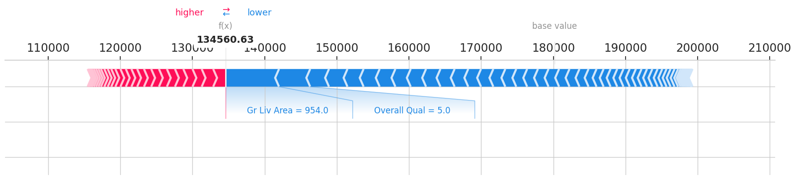
print(f'Prediction for te_data:\n{test_predictions[:10]}\nShape = {test_predictions.shape}')
Prediction for te_data:
array([[134560.62 ],
       [209942.22 ],
       [278879.3  ],
       [125843.02 ],
       [200796.81 ],
       [390743.2  ],
       [158790.19 ],
       [300576.44 ],
       [161224.7  ],
       [ 81361.086]], dtype=float32)
Shape = (411, 1)
[61]:
from sklearn.metrics import mean_absolute_error
print(f'OOF score: {mean_absolute_error(train_data[roles["target"]].values, out_of_fold_predictions.data[:, 0])}')
print(f'HOLDOUT score: {mean_absolute_error(test_data[roles["target"]].values, test_predictions.data[:, 0])}')
OOF score: 13997.699302115092
HOLDOUT score: 12457.17400395377
In the same way as in the previous example with binary classification, you can build a detailed report using ReportDeco, calculate feature importances, use TabularUtilizedAutoML etc.
Shapley values example for regression
Obtaining shapley estimates
[62]:
explainer = SSWARM(automl)
shap_values = explainer.shap_values(test_data, n_jobs=N_THREADS)
100%|████████████████████████████████████████████████████████████████████████████████████████████| 3000/3000 [00:48<00:00, 61.51it/s]
Interpretation plots
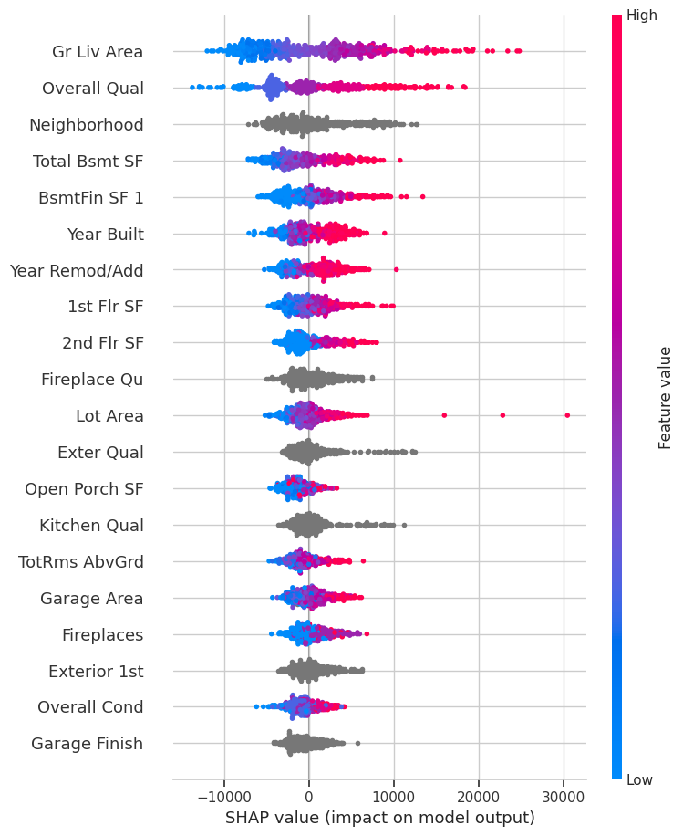
[63]:
# summary plot
shap.summary_plot(shap_values, test_data[explainer.used_feats])
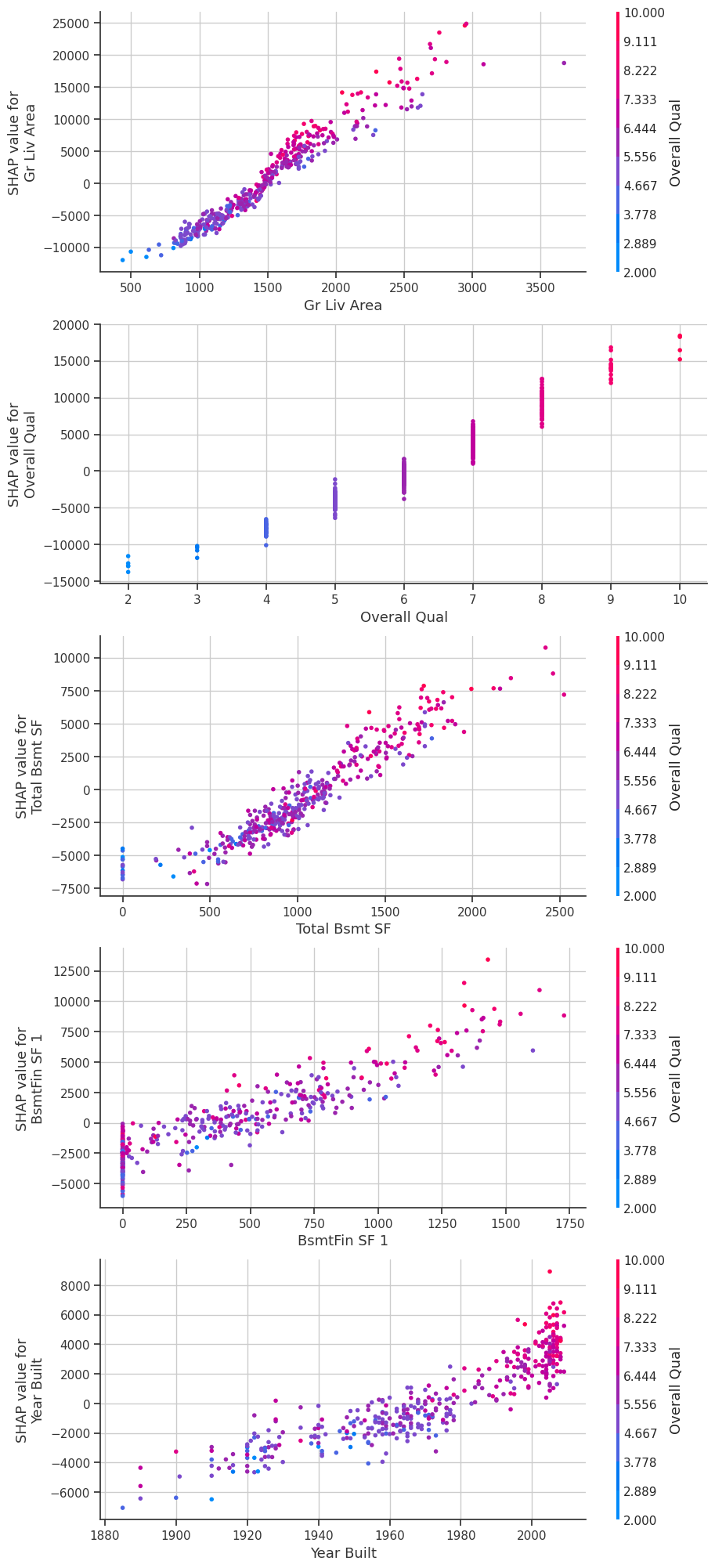
[67]:
# dependence plots
feats = ["Gr Liv Area", "Overall Qual", "Total Bsmt SF", "BsmtFin SF 1", "Year Built"]
fig, ax = plt.subplots(nrows=len(feats), ncols=1, figsize=(10, 5*len(feats)))

for i, feat in enumerate(feats):
    shap.dependence_plot(feat, shap_values, test_data[explainer.used_feats],
                         show=False, ax=ax[i], interaction_index="Overall Qual")
[64]:
# individual force plot
shap.force_plot(explainer.expected_value, shap_values[0], test_data[explainer.used_feats].iloc[0], matplotlib=True)
Multi-class classification
Now let’s consider multi-class classification. Here you will use Anuran Calls (MFCCs) Data Set:
[68]:
from io import BytesIO
from zipfile import ZipFile
from urllib.request import urlopen

data = pd.read_csv(
    ZipFile(
        BytesIO(
            urlopen(
                "https://archive.ics.uci.edu/ml/machine-learning-databases/00406/Anuran%20Calls%20(MFCCs).zip"
            ).read()
        )
    ).open('Frogs_MFCCs.csv')
)

data.head()
[68]:
| MFCCs_ 1 | MFCCs_ 2 | MFCCs_ 3 | MFCCs_ 4 | MFCCs_ 5 | MFCCs_ 6 | MFCCs_ 7 | MFCCs_ 8 | MFCCs_ 9 | MFCCs_10 | ... | MFCCs_17 | MFCCs_18 | MFCCs_19 | MFCCs_20 | MFCCs_21 | MFCCs_22 | Family | Genus | Species | RecordID | |
|---|---|---|---|---|---|---|---|---|---|---|---|---|---|---|---|---|---|---|---|---|---|
| 0 | 1.0 | 0.152936 | -0.105586 | 0.200722 | 0.317201 | 0.260764 | 0.100945 | -0.150063 | -0.171128 | 0.124676 | ... | -0.108351 | -0.077623 | -0.009568 | 0.057684 | 0.118680 | 0.014038 | Leptodactylidae | Adenomera | AdenomeraAndre | 1 |
| 1 | 1.0 | 0.171534 | -0.098975 | 0.268425 | 0.338672 | 0.268353 | 0.060835 | -0.222475 | -0.207693 | 0.170883 | ... | -0.090974 | -0.056510 | -0.035303 | 0.020140 | 0.082263 | 0.029056 | Leptodactylidae | Adenomera | AdenomeraAndre | 1 |
| 2 | 1.0 | 0.152317 | -0.082973 | 0.287128 | 0.276014 | 0.189867 | 0.008714 | -0.242234 | -0.219153 | 0.232538 | ... | -0.050691 | -0.023590 | -0.066722 | -0.025083 | 0.099108 | 0.077162 | Leptodactylidae | Adenomera | AdenomeraAndre | 1 |
| 3 | 1.0 | 0.224392 | 0.118985 | 0.329432 | 0.372088 | 0.361005 | 0.015501 | -0.194347 | -0.098181 | 0.270375 | ... | -0.136009 | -0.177037 | -0.130498 | -0.054766 | -0.018691 | 0.023954 | Leptodactylidae | Adenomera | AdenomeraAndre | 1 |
| 4 | 1.0 | 0.087817 | -0.068345 | 0.306967 | 0.330923 | 0.249144 | 0.006884 | -0.265423 | -0.172700 | 0.266434 | ... | -0.048885 | -0.053074 | -0.088550 | -0.031346 | 0.108610 | 0.079244 | Leptodactylidae | Adenomera | AdenomeraAndre | 1 |
5 rows × 26 columns
[69]:
train_data, test_data = train_test_split(
    data,
    test_size=TEST_SIZE,
    shuffle=True,
    random_state=RANDOM_STATE
)

print(f'Data is splitted. Parts sizes: train_data = {train_data.shape}, test_data = {test_data.shape}')

train_data.head()
Data is splitted. Parts sizes: train_data = (5756, 26), test_data = (1439, 26)
[69]:
| MFCCs_ 1 | MFCCs_ 2 | MFCCs_ 3 | MFCCs_ 4 | MFCCs_ 5 | MFCCs_ 6 | MFCCs_ 7 | MFCCs_ 8 | MFCCs_ 9 | MFCCs_10 | ... | MFCCs_17 | MFCCs_18 | MFCCs_19 | MFCCs_20 | MFCCs_21 | MFCCs_22 | Family | Genus | Species | RecordID | |
|---|---|---|---|---|---|---|---|---|---|---|---|---|---|---|---|---|---|---|---|---|---|
| 3838 | 1.0 | 0.389057 | 0.283855 | 0.558597 | 0.142120 | 0.006777 | -0.100356 | 0.015060 | 0.277700 | 0.062747 | ... | 0.221304 | 0.037511 | -0.019166 | -0.042803 | 0.024793 | 0.177462 | Leptodactylidae | Adenomera | AdenomeraHylaedactylus | 22 |
| 293 | 1.0 | 0.339049 | -0.001276 | 0.075088 | 0.298091 | 0.190639 | 0.022295 | 0.049216 | 0.175380 | -0.007751 | ... | -0.299407 | -0.121592 | 0.108062 | 0.124870 | -0.004888 | -0.040086 | Leptodactylidae | Adenomera | AdenomeraAndre | 7 |
| 1593 | 1.0 | 0.211356 | 0.132368 | 0.530019 | 0.181015 | 0.047415 | -0.142114 | 0.000687 | 0.249328 | 0.032000 | ... | 0.207694 | 0.026302 | -0.167216 | -0.160102 | 0.084770 | 0.276008 | Leptodactylidae | Adenomera | AdenomeraHylaedactylus | 15 |
| 4669 | 1.0 | 0.069635 | 0.170713 | 0.583894 | 0.275507 | 0.086236 | -0.152521 | -0.032355 | 0.268403 | 0.054420 | ... | 0.256234 | -0.116248 | -0.230951 | -0.058546 | 0.205891 | 0.211869 | Leptodactylidae | Adenomera | AdenomeraHylaedactylus | 24 |
| 940 | 1.0 | 0.222777 | -0.069955 | 0.299370 | 0.318585 | 0.094394 | -0.019920 | 0.120537 | 0.192053 | 0.047852 | ... | -0.094684 | -0.104692 | -0.006204 | 0.023067 | -0.044556 | 0.006679 | Dendrobatidae | Ameerega | Ameeregatrivittata | 11 |
5 rows × 26 columns
Now we indicate that we have multi-class classification problem. Default metric and loss is cross-entropy function.
[70]:
task = Task('multiclass')
Set the column roles, build and train AutoML model:
[71]:
roles = {
    'target': 'Species',
    'drop': ['RecordID']

}
[72]:
automl = TabularAutoML(
    task = task,
    timeout = 900,
    cpu_limit = N_THREADS,
    reader_params = {'n_jobs': N_THREADS, 'cv': N_FOLDS, 'random_state': RANDOM_STATE}
)
Note that in case of multi-class classification default pipeline architecture has a slightly different look. First level is the same as level in default binary classification and regression, second level consists of linear regression and LightGBM model and the third is blending. It was decided to use two levels in default architecture based on the results of experiments on different tasks and data, where it gave an increase in model quality. Intuitively, this can be explained by the fact that only at the second and subsequent levels, the model that predicts the probability of belonging to one of the classes can see what the models that predict the rest of the classes see, that is, the models are able to exchange information about classes. Final prediction is blended from last pipeline level.
[73]:
%%time
out_of_fold_predictions = automl.fit_predict(train_data, roles = roles, verbose = 1)
[09:40:33] Stdout logging level is INFO.
[09:40:33] Task: multiclass

[09:40:33] Start automl preset with listed constraints:
[09:40:33] - time: 900.00 seconds
[09:40:33] - CPU: 4 cores
[09:40:33] - memory: 16 GB

[09:40:33] Train data shape: (5756, 26)

[09:40:44] Layer 1 train process start. Time left 889.93 secs
[09:40:44] Start fitting Lvl_0_Pipe_0_Mod_0_LinearL2 ...
[09:40:55] Fitting Lvl_0_Pipe_0_Mod_0_LinearL2 finished. score = -0.010852760572584014
[09:40:55] Lvl_0_Pipe_0_Mod_0_LinearL2 fitting and predicting completed
[09:40:55] Time left 878.58 secs

[09:41:05] Selector_LightGBM fitting and predicting completed
[09:41:05] Start fitting Lvl_0_Pipe_1_Mod_0_LightGBM ...
[09:41:40] Fitting Lvl_0_Pipe_1_Mod_0_LightGBM finished. score = -0.008332313774221245
[09:41:40] Lvl_0_Pipe_1_Mod_0_LightGBM fitting and predicting completed
[09:41:40] Start hyperparameters optimization for Lvl_0_Pipe_1_Mod_1_Tuned_LightGBM ... Time budget is 22.16 secs
[09:42:03] Hyperparameters optimization for Lvl_0_Pipe_1_Mod_1_Tuned_LightGBM completed
[09:42:03] Start fitting Lvl_0_Pipe_1_Mod_1_Tuned_LightGBM ...
The y_pred values do not sum to one. Starting from 1.5 thiswill result in an error.
[09:42:09] Fitting Lvl_0_Pipe_1_Mod_1_Tuned_LightGBM finished. score = -0.006176167581894699
[09:42:09] Lvl_0_Pipe_1_Mod_1_Tuned_LightGBM fitting and predicting completed
[09:42:09] Start fitting Lvl_0_Pipe_1_Mod_2_CatBoost ...
The y_pred values do not sum to one. Starting from 1.5 thiswill result in an error.
[09:42:39] Fitting Lvl_0_Pipe_1_Mod_2_CatBoost finished. score = -0.0052738622218159725
[09:42:39] Lvl_0_Pipe_1_Mod_2_CatBoost fitting and predicting completed
[09:42:39] Start hyperparameters optimization for Lvl_0_Pipe_1_Mod_3_Tuned_CatBoost ... Time budget is 290.54 secs
The y_pred values do not sum to one. Starting from 1.5 thiswill result in an error.
The y_pred values do not sum to one. Starting from 1.5 thiswill result in an error.
The y_pred values do not sum to one. Starting from 1.5 thiswill result in an error.
The y_pred values do not sum to one. Starting from 1.5 thiswill result in an error.
The y_pred values do not sum to one. Starting from 1.5 thiswill result in an error.
The y_pred values do not sum to one. Starting from 1.5 thiswill result in an error.
The y_pred values do not sum to one. Starting from 1.5 thiswill result in an error.
The y_pred values do not sum to one. Starting from 1.5 thiswill result in an error.
The y_pred values do not sum to one. Starting from 1.5 thiswill result in an error.
The y_pred values do not sum to one. Starting from 1.5 thiswill result in an error.
The y_pred values do not sum to one. Starting from 1.5 thiswill result in an error.
The y_pred values do not sum to one. Starting from 1.5 thiswill result in an error.
The y_pred values do not sum to one. Starting from 1.5 thiswill result in an error.
The y_pred values do not sum to one. Starting from 1.5 thiswill result in an error.
The y_pred values do not sum to one. Starting from 1.5 thiswill result in an error.
The y_pred values do not sum to one. Starting from 1.5 thiswill result in an error.
The y_pred values do not sum to one. Starting from 1.5 thiswill result in an error.
The y_pred values do not sum to one. Starting from 1.5 thiswill result in an error.
[09:47:31] Hyperparameters optimization for Lvl_0_Pipe_1_Mod_3_Tuned_CatBoost completed
[09:47:31] Start fitting Lvl_0_Pipe_1_Mod_3_Tuned_CatBoost ...
[09:48:36] Fitting Lvl_0_Pipe_1_Mod_3_Tuned_CatBoost finished. score = -0.004565362115455095
[09:48:36] Lvl_0_Pipe_1_Mod_3_Tuned_CatBoost fitting and predicting completed
[09:48:36] Time left 417.56 secs

[09:48:36] Layer 1 training completed.

[09:48:36] Layer 2 train process start. Time left 417.53 secs
The y_pred values do not sum to one. Starting from 1.5 thiswill result in an error.
[09:48:36] Start fitting Lvl_1_Pipe_0_Mod_0_LinearL2 ...
[09:48:45] Fitting Lvl_1_Pipe_0_Mod_0_LinearL2 finished. score = -0.006018851790978736
[09:48:45] Lvl_1_Pipe_0_Mod_0_LinearL2 fitting and predicting completed
[09:48:45] Time left 408.00 secs

[09:48:46] Start fitting Lvl_1_Pipe_1_Mod_0_LightGBM ...
[09:49:32] Fitting Lvl_1_Pipe_1_Mod_0_LightGBM finished. score = -0.005526817945493392
[09:49:32] Lvl_1_Pipe_1_Mod_0_LightGBM fitting and predicting completed
[09:49:32] Time left 361.18 secs

[09:49:32] Layer 2 training completed.

[09:49:32] Blending: optimization starts with equal weights and score -0.005530615286885703
[09:49:32] Blending: iteration 0: score = -0.005432028962983418, weights = [0.1987539 0.8012461]
[09:49:32] Blending: iteration 1: score = -0.005432028962983418, weights = [0.1987539 0.8012461]
[09:49:32] Blending: no score update. Terminated

[09:49:32] Automl preset training completed in 539.00 seconds

[09:49:32] Model description:
Models on level 0:
         5 averaged models Lvl_0_Pipe_0_Mod_0_LinearL2
         5 averaged models Lvl_0_Pipe_1_Mod_0_LightGBM
         5 averaged models Lvl_0_Pipe_1_Mod_1_Tuned_LightGBM
         5 averaged models Lvl_0_Pipe_1_Mod_2_CatBoost
         5 averaged models Lvl_0_Pipe_1_Mod_3_Tuned_CatBoost

Final prediction for new objects (level 1) =
         0.19875 * (5 averaged models Lvl_1_Pipe_0_Mod_0_LinearL2) +
         0.80125 * (5 averaged models Lvl_1_Pipe_1_Mod_0_LightGBM)

CPU times: user 32min 14s, sys: 1min 22s, total: 33min 36s
Wall time: 8min 59s
[74]:
%%time

test_predictions = automl.predict(test_data)
print(f'Prediction for test_data:\n{test_predictions}\nShape = {test_predictions.shape}')
Prediction for test_data:
array([[9.9961942e-01, 9.1690832e-05, 4.9272418e-05, ..., 2.9182707e-05,
        2.1924083e-05, 1.8040057e-05],
       [7.2180563e-05, 4.8093905e-05, 6.2713400e-05, ..., 3.6562527e-05,
        3.1231004e-05, 2.4088009e-05],
       [1.0252791e-04, 9.9920928e-01, 1.0877274e-04, ..., 6.9528498e-05,
        4.4692573e-05, 3.8138864e-05],
       ...,
       [2.8551594e-04, 1.0709166e-04, 9.9875408e-01, ..., 9.3088362e-05,
        7.5856973e-05, 6.2510102e-05],
       [2.2101802e-04, 7.7087658e-05, 9.9894643e-01, ..., 9.0580215e-05,
        7.7611970e-05, 6.3799351e-05],
       [1.2458056e-04, 9.9910909e-01, 9.0568836e-05, ..., 5.4615561e-05,
        4.9981187e-05, 3.5048710e-05]], dtype=float32)
Shape = (1439, 10)
CPU times: user 8.35 s, sys: 469 ms, total: 8.82 s
Wall time: 2.21 s
It is also important to note that the Reader object may re-label classes during training. To see the new labelling, you can call .class_mapping method of Reader object. If the output dict is empty, then the original order and class layout has been preserved.
[75]:
automl.reader.class_mapping
[75]:
{'AdenomeraHylaedactylus': 0,
 'HypsiboasCordobae': 1,
 'AdenomeraAndre': 2,
 'Ameeregatrivittata': 3,
 'HypsiboasCinerascens': 4,
 'HylaMinuta': 5,
 'LeptodactylusFuscus': 6,
 'ScinaxRuber': 7,
 'OsteocephalusOophagus': 8,
 'Rhinellagranulosa': 9}
Just in case, in order to avoid problems, it is better to relabel known class labels when calculating metrics, for example, in this or similar way:
[76]:
mapping = automl.reader.class_mapping
def map_class(x):
    return mapping[x]

mapped = np.vectorize(map_class)
mapped(train_data['Species'].values)
[76]:
array([0, 2, 0, ..., 4, 4, 3])
[77]:
from sklearn.metrics import log_loss
print(f'OOF score: {log_loss(mapped(train_data[roles["target"]].values), out_of_fold_predictions.data)}')
print(f'HOLDOUT score: {log_loss(mapped(test_data[roles["target"]].values), test_predictions.data)}')
OOF score: 0.005432028962983418
HOLDOUT score: 0.0014346529369004119
Feature importance calculation, building reports, time management etc are also available for multiclass classification.
Multi-label classification
Now let’s consider multi-label classification task, here you will use the same dataset as in section above (Anuran Calls (MFCCs) Data Set ). Let’s pick labels in each column:
[78]:
data['AdenomeraHylaedactylus'] = (data['Species'] == 'AdenomeraHylaedactylus').astype(int)
data['Adenomera'] = (data['Genus'] == 'Adenomera').astype(int)
data['Leptodactylidae'] = (data['Family'] == 'Leptodactylidae').astype(int)
[79]:
data.head()
[79]:
| MFCCs_ 1 | MFCCs_ 2 | MFCCs_ 3 | MFCCs_ 4 | MFCCs_ 5 | MFCCs_ 6 | MFCCs_ 7 | MFCCs_ 8 | MFCCs_ 9 | MFCCs_10 | ... | MFCCs_20 | MFCCs_21 | MFCCs_22 | Family | Genus | Species | RecordID | AdenomeraHylaedactylus | Adenomera | Leptodactylidae | |
|---|---|---|---|---|---|---|---|---|---|---|---|---|---|---|---|---|---|---|---|---|---|
| 0 | 1.0 | 0.152936 | -0.105586 | 0.200722 | 0.317201 | 0.260764 | 0.100945 | -0.150063 | -0.171128 | 0.124676 | ... | 0.057684 | 0.118680 | 0.014038 | Leptodactylidae | Adenomera | AdenomeraAndre | 1 | 0 | 1 | 1 |
| 1 | 1.0 | 0.171534 | -0.098975 | 0.268425 | 0.338672 | 0.268353 | 0.060835 | -0.222475 | -0.207693 | 0.170883 | ... | 0.020140 | 0.082263 | 0.029056 | Leptodactylidae | Adenomera | AdenomeraAndre | 1 | 0 | 1 | 1 |
| 2 | 1.0 | 0.152317 | -0.082973 | 0.287128 | 0.276014 | 0.189867 | 0.008714 | -0.242234 | -0.219153 | 0.232538 | ... | -0.025083 | 0.099108 | 0.077162 | Leptodactylidae | Adenomera | AdenomeraAndre | 1 | 0 | 1 | 1 |
| 3 | 1.0 | 0.224392 | 0.118985 | 0.329432 | 0.372088 | 0.361005 | 0.015501 | -0.194347 | -0.098181 | 0.270375 | ... | -0.054766 | -0.018691 | 0.023954 | Leptodactylidae | Adenomera | AdenomeraAndre | 1 | 0 | 1 | 1 |
| 4 | 1.0 | 0.087817 | -0.068345 | 0.306967 | 0.330923 | 0.249144 | 0.006884 | -0.265423 | -0.172700 | 0.266434 | ... | -0.031346 | 0.108610 | 0.079244 | Leptodactylidae | Adenomera | AdenomeraAndre | 1 | 0 | 1 | 1 |
5 rows × 29 columns
[80]:
targets = ['Leptodactylidae', 'Adenomera', 'AdenomeraHylaedactylus']
Split it to train and validation:
[81]:
train_data, test_data = train_test_split(
    data,
    test_size=TEST_SIZE,
    random_state=RANDOM_STATE
)

print(f'Data is splitted. Parts sizes: train_data = {train_data.shape}, test_data = {test_data.shape}')

train_data.head()
Data is splitted. Parts sizes: train_data = (5756, 29), test_data = (1439, 29)
[81]:
| MFCCs_ 1 | MFCCs_ 2 | MFCCs_ 3 | MFCCs_ 4 | MFCCs_ 5 | MFCCs_ 6 | MFCCs_ 7 | MFCCs_ 8 | MFCCs_ 9 | MFCCs_10 | ... | MFCCs_20 | MFCCs_21 | MFCCs_22 | Family | Genus | Species | RecordID | AdenomeraHylaedactylus | Adenomera | Leptodactylidae | |
|---|---|---|---|---|---|---|---|---|---|---|---|---|---|---|---|---|---|---|---|---|---|
| 3838 | 1.0 | 0.389057 | 0.283855 | 0.558597 | 0.142120 | 0.006777 | -0.100356 | 0.015060 | 0.277700 | 0.062747 | ... | -0.042803 | 0.024793 | 0.177462 | Leptodactylidae | Adenomera | AdenomeraHylaedactylus | 22 | 1 | 1 | 1 |
| 293 | 1.0 | 0.339049 | -0.001276 | 0.075088 | 0.298091 | 0.190639 | 0.022295 | 0.049216 | 0.175380 | -0.007751 | ... | 0.124870 | -0.004888 | -0.040086 | Leptodactylidae | Adenomera | AdenomeraAndre | 7 | 0 | 1 | 1 |
| 1593 | 1.0 | 0.211356 | 0.132368 | 0.530019 | 0.181015 | 0.047415 | -0.142114 | 0.000687 | 0.249328 | 0.032000 | ... | -0.160102 | 0.084770 | 0.276008 | Leptodactylidae | Adenomera | AdenomeraHylaedactylus | 15 | 1 | 1 | 1 |
| 4669 | 1.0 | 0.069635 | 0.170713 | 0.583894 | 0.275507 | 0.086236 | -0.152521 | -0.032355 | 0.268403 | 0.054420 | ... | -0.058546 | 0.205891 | 0.211869 | Leptodactylidae | Adenomera | AdenomeraHylaedactylus | 24 | 1 | 1 | 1 |
| 940 | 1.0 | 0.222777 | -0.069955 | 0.299370 | 0.318585 | 0.094394 | -0.019920 | 0.120537 | 0.192053 | 0.047852 | ... | 0.023067 | -0.044556 | 0.006679 | Dendrobatidae | Ameerega | Ameeregatrivittata | 11 | 0 | 0 | 0 |
5 rows × 29 columns
Indicate that we are solving multi-label classification problem. Default metric and loss for this task is logloss.
[82]:
task = Task('multilabel')
multilabel isn`t supported in lgb
Specifying the roles. Now we have several columns with target variables, and it’s necessary to specify them all.
[83]:
roles = {
    'target': ['Leptodactylidae', 'Adenomera', 'AdenomeraHylaedactylus'],
    'drop': ['RecordID', 'Species', 'Genus', 'Family']
}
Create TabularAutoML instance. One of the differences in this case is that by default, random forest algorithm will be used at the end before blending.
[84]:
automl = TabularAutoML(
    task = task,
    timeout = 3600,
    cpu_limit = N_THREADS,
    reader_params = {'n_jobs': N_THREADS, 'cv': N_FOLDS, 'random_state': RANDOM_STATE}, #TODO: N_THREADS
    general_params = {'use_algos': 'auto'}
)
Training:
[85]:
%%time
out_of_fold_predictions = automl.fit_predict(train_data, roles = roles, verbose = 1)
[09:49:35] Stdout logging level is INFO.
[09:49:35] Task: multilabel

[09:49:35] Start automl preset with listed constraints:
[09:49:35] - time: 3600.00 seconds
[09:49:35] - CPU: 4 cores
[09:49:35] - memory: 16 GB

[09:49:35] Train data shape: (5756, 29)

[09:49:39] Layer 1 train process start. Time left 3595.80 secs
[09:49:39] Start fitting Lvl_0_Pipe_0_Mod_0_RFSklearn ...
The y_pred values do not sum to one. Starting from 1.5 thiswill result in an error.
The y_pred values do not sum to one. Starting from 1.5 thiswill result in an error.
The y_pred values do not sum to one. Starting from 1.5 thiswill result in an error.
The y_pred values do not sum to one. Starting from 1.5 thiswill result in an error.
[09:50:17] Fitting Lvl_0_Pipe_0_Mod_0_RFSklearn finished. score = -1.7417950747859665
[09:50:17] Lvl_0_Pipe_0_Mod_0_RFSklearn fitting and predicting completed
[09:50:17] Start hyperparameters optimization for Lvl_0_Pipe_0_Mod_1_Tuned_RFSklearn ... Time budget is 300.00 secs
The y_pred values do not sum to one. Starting from 1.5 thiswill result in an error.
The y_pred values do not sum to one. Starting from 1.5 thiswill result in an error.
The y_pred values do not sum to one. Starting from 1.5 thiswill result in an error.
The y_pred values do not sum to one. Starting from 1.5 thiswill result in an error.
The y_pred values do not sum to one. Starting from 1.5 thiswill result in an error.
The y_pred values do not sum to one. Starting from 1.5 thiswill result in an error.
The y_pred values do not sum to one. Starting from 1.5 thiswill result in an error.
The y_pred values do not sum to one. Starting from 1.5 thiswill result in an error.
The y_pred values do not sum to one. Starting from 1.5 thiswill result in an error.
The y_pred values do not sum to one. Starting from 1.5 thiswill result in an error.
The y_pred values do not sum to one. Starting from 1.5 thiswill result in an error.
The y_pred values do not sum to one. Starting from 1.5 thiswill result in an error.
The y_pred values do not sum to one. Starting from 1.5 thiswill result in an error.
The y_pred values do not sum to one. Starting from 1.5 thiswill result in an error.
The y_pred values do not sum to one. Starting from 1.5 thiswill result in an error.
The y_pred values do not sum to one. Starting from 1.5 thiswill result in an error.
The y_pred values do not sum to one. Starting from 1.5 thiswill result in an error.
The y_pred values do not sum to one. Starting from 1.5 thiswill result in an error.
The y_pred values do not sum to one. Starting from 1.5 thiswill result in an error.
The y_pred values do not sum to one. Starting from 1.5 thiswill result in an error.
The y_pred values do not sum to one. Starting from 1.5 thiswill result in an error.
The y_pred values do not sum to one. Starting from 1.5 thiswill result in an error.
The y_pred values do not sum to one. Starting from 1.5 thiswill result in an error.
The y_pred values do not sum to one. Starting from 1.5 thiswill result in an error.
The y_pred values do not sum to one. Starting from 1.5 thiswill result in an error.
The y_pred values do not sum to one. Starting from 1.5 thiswill result in an error.
The y_pred values do not sum to one. Starting from 1.5 thiswill result in an error.
The y_pred values do not sum to one. Starting from 1.5 thiswill result in an error.
The y_pred values do not sum to one. Starting from 1.5 thiswill result in an error.
The y_pred values do not sum to one. Starting from 1.5 thiswill result in an error.
The y_pred values do not sum to one. Starting from 1.5 thiswill result in an error.
The y_pred values do not sum to one. Starting from 1.5 thiswill result in an error.
The y_pred values do not sum to one. Starting from 1.5 thiswill result in an error.
The y_pred values do not sum to one. Starting from 1.5 thiswill result in an error.
The y_pred values do not sum to one. Starting from 1.5 thiswill result in an error.
The y_pred values do not sum to one. Starting from 1.5 thiswill result in an error.
The y_pred values do not sum to one. Starting from 1.5 thiswill result in an error.
The y_pred values do not sum to one. Starting from 1.5 thiswill result in an error.
The y_pred values do not sum to one. Starting from 1.5 thiswill result in an error.
The y_pred values do not sum to one. Starting from 1.5 thiswill result in an error.
The y_pred values do not sum to one. Starting from 1.5 thiswill result in an error.
The y_pred values do not sum to one. Starting from 1.5 thiswill result in an error.
The y_pred values do not sum to one. Starting from 1.5 thiswill result in an error.
The y_pred values do not sum to one. Starting from 1.5 thiswill result in an error.
The y_pred values do not sum to one. Starting from 1.5 thiswill result in an error.
The y_pred values do not sum to one. Starting from 1.5 thiswill result in an error.
The y_pred values do not sum to one. Starting from 1.5 thiswill result in an error.
The y_pred values do not sum to one. Starting from 1.5 thiswill result in an error.
The y_pred values do not sum to one. Starting from 1.5 thiswill result in an error.
The y_pred values do not sum to one. Starting from 1.5 thiswill result in an error.
The y_pred values do not sum to one. Starting from 1.5 thiswill result in an error.
The y_pred values do not sum to one. Starting from 1.5 thiswill result in an error.
The y_pred values do not sum to one. Starting from 1.5 thiswill result in an error.
The y_pred values do not sum to one. Starting from 1.5 thiswill result in an error.
The y_pred values do not sum to one. Starting from 1.5 thiswill result in an error.
The y_pred values do not sum to one. Starting from 1.5 thiswill result in an error.
The y_pred values do not sum to one. Starting from 1.5 thiswill result in an error.
The y_pred values do not sum to one. Starting from 1.5 thiswill result in an error.
The y_pred values do not sum to one. Starting from 1.5 thiswill result in an error.
The y_pred values do not sum to one. Starting from 1.5 thiswill result in an error.
The y_pred values do not sum to one. Starting from 1.5 thiswill result in an error.
The y_pred values do not sum to one. Starting from 1.5 thiswill result in an error.
The y_pred values do not sum to one. Starting from 1.5 thiswill result in an error.
The y_pred values do not sum to one. Starting from 1.5 thiswill result in an error.
The y_pred values do not sum to one. Starting from 1.5 thiswill result in an error.
The y_pred values do not sum to one. Starting from 1.5 thiswill result in an error.
The y_pred values do not sum to one. Starting from 1.5 thiswill result in an error.
The y_pred values do not sum to one. Starting from 1.5 thiswill result in an error.
The y_pred values do not sum to one. Starting from 1.5 thiswill result in an error.
The y_pred values do not sum to one. Starting from 1.5 thiswill result in an error.
The y_pred values do not sum to one. Starting from 1.5 thiswill result in an error.
The y_pred values do not sum to one. Starting from 1.5 thiswill result in an error.
The y_pred values do not sum to one. Starting from 1.5 thiswill result in an error.
The y_pred values do not sum to one. Starting from 1.5 thiswill result in an error.
The y_pred values do not sum to one. Starting from 1.5 thiswill result in an error.
The y_pred values do not sum to one. Starting from 1.5 thiswill result in an error.
The y_pred values do not sum to one. Starting from 1.5 thiswill result in an error.
The y_pred values do not sum to one. Starting from 1.5 thiswill result in an error.
The y_pred values do not sum to one. Starting from 1.5 thiswill result in an error.
The y_pred values do not sum to one. Starting from 1.5 thiswill result in an error.
[09:55:22] Hyperparameters optimization for Lvl_0_Pipe_0_Mod_1_Tuned_RFSklearn completed
[09:55:22] Start fitting Lvl_0_Pipe_0_Mod_1_Tuned_RFSklearn ...
[09:55:22] Time left 3253.57 secs

[09:55:22] Start fitting Lvl_0_Pipe_1_Mod_0_LinearL2 ...
The y_pred values do not sum to one. Starting from 1.5 thiswill result in an error.
The y_pred values do not sum to one. Starting from 1.5 thiswill result in an error.
The y_pred values do not sum to one. Starting from 1.5 thiswill result in an error.
The y_pred values do not sum to one. Starting from 1.5 thiswill result in an error.
The y_pred values do not sum to one. Starting from 1.5 thiswill result in an error.
The y_pred values do not sum to one. Starting from 1.5 thiswill result in an error.
The y_pred values do not sum to one. Starting from 1.5 thiswill result in an error.
The y_pred values do not sum to one. Starting from 1.5 thiswill result in an error.
The y_pred values do not sum to one. Starting from 1.5 thiswill result in an error.
The y_pred values do not sum to one. Starting from 1.5 thiswill result in an error.
The y_pred values do not sum to one. Starting from 1.5 thiswill result in an error.
The y_pred values do not sum to one. Starting from 1.5 thiswill result in an error.
The y_pred values do not sum to one. Starting from 1.5 thiswill result in an error.
The y_pred values do not sum to one. Starting from 1.5 thiswill result in an error.
The y_pred values do not sum to one. Starting from 1.5 thiswill result in an error.
The y_pred values do not sum to one. Starting from 1.5 thiswill result in an error.
The y_pred values do not sum to one. Starting from 1.5 thiswill result in an error.
The y_pred values do not sum to one. Starting from 1.5 thiswill result in an error.
The y_pred values do not sum to one. Starting from 1.5 thiswill result in an error.
The y_pred values do not sum to one. Starting from 1.5 thiswill result in an error.
The y_pred values do not sum to one. Starting from 1.5 thiswill result in an error.
The y_pred values do not sum to one. Starting from 1.5 thiswill result in an error.
The y_pred values do not sum to one. Starting from 1.5 thiswill result in an error.
The y_pred values do not sum to one. Starting from 1.5 thiswill result in an error.
The y_pred values do not sum to one. Starting from 1.5 thiswill result in an error.
The y_pred values do not sum to one. Starting from 1.5 thiswill result in an error.
The y_pred values do not sum to one. Starting from 1.5 thiswill result in an error.
The y_pred values do not sum to one. Starting from 1.5 thiswill result in an error.
The y_pred values do not sum to one. Starting from 1.5 thiswill result in an error.
The y_pred values do not sum to one. Starting from 1.5 thiswill result in an error.
The y_pred values do not sum to one. Starting from 1.5 thiswill result in an error.
The y_pred values do not sum to one. Starting from 1.5 thiswill result in an error.
The y_pred values do not sum to one. Starting from 1.5 thiswill result in an error.
The y_pred values do not sum to one. Starting from 1.5 thiswill result in an error.
The y_pred values do not sum to one. Starting from 1.5 thiswill result in an error.
The y_pred values do not sum to one. Starting from 1.5 thiswill result in an error.
The y_pred values do not sum to one. Starting from 1.5 thiswill result in an error.
The y_pred values do not sum to one. Starting from 1.5 thiswill result in an error.
The y_pred values do not sum to one. Starting from 1.5 thiswill result in an error.
The y_pred values do not sum to one. Starting from 1.5 thiswill result in an error.
The y_pred values do not sum to one. Starting from 1.5 thiswill result in an error.
The y_pred values do not sum to one. Starting from 1.5 thiswill result in an error.
The y_pred values do not sum to one. Starting from 1.5 thiswill result in an error.
The y_pred values do not sum to one. Starting from 1.5 thiswill result in an error.
The y_pred values do not sum to one. Starting from 1.5 thiswill result in an error.
The y_pred values do not sum to one. Starting from 1.5 thiswill result in an error.
The y_pred values do not sum to one. Starting from 1.5 thiswill result in an error.
The y_pred values do not sum to one. Starting from 1.5 thiswill result in an error.
The y_pred values do not sum to one. Starting from 1.5 thiswill result in an error.
The y_pred values do not sum to one. Starting from 1.5 thiswill result in an error.
[09:55:27] Fitting Lvl_0_Pipe_1_Mod_0_LinearL2 finished. score = -1.7293712480945589
[09:55:27] Lvl_0_Pipe_1_Mod_0_LinearL2 fitting and predicting completed
[09:55:27] Time left 3248.38 secs
The y_pred values do not sum to one. Starting from 1.5 thiswill result in an error.
The y_pred values do not sum to one. Starting from 1.5 thiswill result in an error.
[09:55:39] Selector_CatBoost fitting and predicting completed
[09:55:39] Start fitting Lvl_0_Pipe_2_Mod_0_CatBoost ...
[09:56:19] Fitting Lvl_0_Pipe_2_Mod_0_CatBoost finished. score = -1.7239793390118887
[09:56:19] Lvl_0_Pipe_2_Mod_0_CatBoost fitting and predicting completed
[09:56:19] Start hyperparameters optimization for Lvl_0_Pipe_2_Mod_1_Tuned_CatBoost ... Time budget is 300.00 secs
The y_pred values do not sum to one. Starting from 1.5 thiswill result in an error.
The y_pred values do not sum to one. Starting from 1.5 thiswill result in an error.
The y_pred values do not sum to one. Starting from 1.5 thiswill result in an error.
The y_pred values do not sum to one. Starting from 1.5 thiswill result in an error.
The y_pred values do not sum to one. Starting from 1.5 thiswill result in an error.
The y_pred values do not sum to one. Starting from 1.5 thiswill result in an error.
The y_pred values do not sum to one. Starting from 1.5 thiswill result in an error.
The y_pred values do not sum to one. Starting from 1.5 thiswill result in an error.
The y_pred values do not sum to one. Starting from 1.5 thiswill result in an error.
The y_pred values do not sum to one. Starting from 1.5 thiswill result in an error.
The y_pred values do not sum to one. Starting from 1.5 thiswill result in an error.
The y_pred values do not sum to one. Starting from 1.5 thiswill result in an error.
The y_pred values do not sum to one. Starting from 1.5 thiswill result in an error.
The y_pred values do not sum to one. Starting from 1.5 thiswill result in an error.
The y_pred values do not sum to one. Starting from 1.5 thiswill result in an error.
[10:01:29] Hyperparameters optimization for Lvl_0_Pipe_2_Mod_1_Tuned_CatBoost completed
[10:01:29] Start fitting Lvl_0_Pipe_2_Mod_1_Tuned_CatBoost ...
The y_pred values do not sum to one. Starting from 1.5 thiswill result in an error.
[10:03:35] Fitting Lvl_0_Pipe_2_Mod_1_Tuned_CatBoost finished. score = -1.7234197039272048
[10:03:35] Lvl_0_Pipe_2_Mod_1_Tuned_CatBoost fitting and predicting completed
[10:03:35] Time left 2759.75 secs

[10:03:35] Layer 1 training completed.

[10:03:35] Blending: optimization starts with equal weights and score -1.7268388233390646
The y_pred values do not sum to one. Starting from 1.5 thiswill result in an error.
The y_pred values do not sum to one. Starting from 1.5 thiswill result in an error.
The y_pred values do not sum to one. Starting from 1.5 thiswill result in an error.
The y_pred values do not sum to one. Starting from 1.5 thiswill result in an error.
The y_pred values do not sum to one. Starting from 1.5 thiswill result in an error.
The y_pred values do not sum to one. Starting from 1.5 thiswill result in an error.
The y_pred values do not sum to one. Starting from 1.5 thiswill result in an error.
The y_pred values do not sum to one. Starting from 1.5 thiswill result in an error.
The y_pred values do not sum to one. Starting from 1.5 thiswill result in an error.
The y_pred values do not sum to one. Starting from 1.5 thiswill result in an error.
The y_pred values do not sum to one. Starting from 1.5 thiswill result in an error.
The y_pred values do not sum to one. Starting from 1.5 thiswill result in an error.
The y_pred values do not sum to one. Starting from 1.5 thiswill result in an error.
The y_pred values do not sum to one. Starting from 1.5 thiswill result in an error.
The y_pred values do not sum to one. Starting from 1.5 thiswill result in an error.
The y_pred values do not sum to one. Starting from 1.5 thiswill result in an error.
The y_pred values do not sum to one. Starting from 1.5 thiswill result in an error.
The y_pred values do not sum to one. Starting from 1.5 thiswill result in an error.
The y_pred values do not sum to one. Starting from 1.5 thiswill result in an error.
The y_pred values do not sum to one. Starting from 1.5 thiswill result in an error.
The y_pred values do not sum to one. Starting from 1.5 thiswill result in an error.
The y_pred values do not sum to one. Starting from 1.5 thiswill result in an error.
The y_pred values do not sum to one. Starting from 1.5 thiswill result in an error.
The y_pred values do not sum to one. Starting from 1.5 thiswill result in an error.
The y_pred values do not sum to one. Starting from 1.5 thiswill result in an error.
The y_pred values do not sum to one. Starting from 1.5 thiswill result in an error.
The y_pred values do not sum to one. Starting from 1.5 thiswill result in an error.
The y_pred values do not sum to one. Starting from 1.5 thiswill result in an error.
The y_pred values do not sum to one. Starting from 1.5 thiswill result in an error.
[10:03:36] Blending: iteration 0: score = -1.723183644831893, weights = [0. 0. 0.4463267 0.55367327]
The y_pred values do not sum to one. Starting from 1.5 thiswill result in an error.
The y_pred values do not sum to one. Starting from 1.5 thiswill result in an error.
The y_pred values do not sum to one. Starting from 1.5 thiswill result in an error.
The y_pred values do not sum to one. Starting from 1.5 thiswill result in an error.
The y_pred values do not sum to one. Starting from 1.5 thiswill result in an error.
The y_pred values do not sum to one. Starting from 1.5 thiswill result in an error.
The y_pred values do not sum to one. Starting from 1.5 thiswill result in an error.
The y_pred values do not sum to one. Starting from 1.5 thiswill result in an error.
The y_pred values do not sum to one. Starting from 1.5 thiswill result in an error.
The y_pred values do not sum to one. Starting from 1.5 thiswill result in an error.
The y_pred values do not sum to one. Starting from 1.5 thiswill result in an error.
The y_pred values do not sum to one. Starting from 1.5 thiswill result in an error.
The y_pred values do not sum to one. Starting from 1.5 thiswill result in an error.
The y_pred values do not sum to one. Starting from 1.5 thiswill result in an error.
The y_pred values do not sum to one. Starting from 1.5 thiswill result in an error.
The y_pred values do not sum to one. Starting from 1.5 thiswill result in an error.
The y_pred values do not sum to one. Starting from 1.5 thiswill result in an error.
The y_pred values do not sum to one. Starting from 1.5 thiswill result in an error.
The y_pred values do not sum to one. Starting from 1.5 thiswill result in an error.
The y_pred values do not sum to one. Starting from 1.5 thiswill result in an error.
The y_pred values do not sum to one. Starting from 1.5 thiswill result in an error.
The y_pred values do not sum to one. Starting from 1.5 thiswill result in an error.
The y_pred values do not sum to one. Starting from 1.5 thiswill result in an error.
The y_pred values do not sum to one. Starting from 1.5 thiswill result in an error.
The y_pred values do not sum to one. Starting from 1.5 thiswill result in an error.
The y_pred values do not sum to one. Starting from 1.5 thiswill result in an error.
The y_pred values do not sum to one. Starting from 1.5 thiswill result in an error.
The y_pred values do not sum to one. Starting from 1.5 thiswill result in an error.
The y_pred values do not sum to one. Starting from 1.5 thiswill result in an error.
[10:03:36] Blending: iteration 1: score = -1.723183644831893, weights = [0.         0.         0.4463267  0.55367327]
[10:03:36] Blending: no score update. Terminated

[10:03:36] Automl preset training completed in 840.67 seconds

[10:03:36] Model description:
Final prediction for new objects (level 0) =
         0.44633 * (5 averaged models Lvl_0_Pipe_2_Mod_0_CatBoost) +
         0.55367 * (5 averaged models Lvl_0_Pipe_2_Mod_1_Tuned_CatBoost)

CPU times: user 40min 39s, sys: 3min 26s, total: 44min 5s
Wall time: 14min
Get a prediction on the test data:
[86]:
%%time

test_predictions = automl.predict(test_data)
print(f'Prediction for test_data:\n{test_predictions}\nShape = {test_predictions.shape}')
Prediction for test_data:
array([[9.9938047e-01, 9.9943602e-01, 9.9970806e-01],
       [2.3319555e-04, 1.4785888e-04, 3.1775104e-05],
       [3.7830789e-04, 4.8983089e-05, 5.8558126e-06],
       ...,
       [9.1259861e-01, 9.2034292e-01, 1.7304690e-05],
       [9.9985009e-01, 9.9985689e-01, 2.9136087e-05],
       [8.1000919e-04, 1.9849822e-04, 3.6050700e-05]], dtype=float32)
Shape = (1439, 3)
CPU times: user 1.15 s, sys: 178 ms, total: 1.33 s
Wall time: 185 ms
Note that in case of multi-label classification classes order always remains unchanged.
[87]:
automl.reader.class_mapping
[87]:
{'Leptodactylidae': None, 'Adenomera': None, 'AdenomeraHylaedactylus': None}
It is importatnt to note that in this case models taken in the final composition did not have time to learn on all cross-validation folds, so their predicts in them will be NaNs:
[88]:
np.unique(np.isnan(out_of_fold_predictions.data))
[88]:
array([False])
But for new data, normal numerical predictions are made:
[89]:
np.unique(np.isnan(test_predictions.data))
[89]:
array([False])
Therefore, we can calculate the logloss from sklearn only on the test set (because of NaNs):
[90]:
from sklearn.metrics import log_loss
print(f'HOLDOUT score: {log_loss(test_data[targets].values, test_predictions.data)}')
HOLDOUT score: 1.7310181043031334
The y_pred values do not sum to one. Starting from 1.5 thiswill result in an error.
Multi-output regression
For completeness, let’s consider multi-output regression task. Here you will use Energy Efficiency dataset.
Data loading and splitting:
[94]:
columns = [
    'relative_compactness', 'surface_area', 'wall_area', 'roof_area',
    'overall_height', 'orientation', 'glazing_area',
    'glazing_area_distribution', 'heating_load', 'cooling_load'
]
data = pd.read_excel("https://archive.ics.uci.edu/ml/machine-learning-databases/00242/ENB2012_data.xlsx", names=columns, header=None)
data = data.drop(index=0, inplace=False)
data
[94]:
| relative_compactness | surface_area | wall_area | roof_area | overall_height | orientation | glazing_area | glazing_area_distribution | heating_load | cooling_load | |
|---|---|---|---|---|---|---|---|---|---|---|
| 1 | 0.98 | 514.5 | 294 | 110.25 | 7 | 2 | 0 | 0 | 15.55 | 21.33 |
| 2 | 0.98 | 514.5 | 294 | 110.25 | 7 | 3 | 0 | 0 | 15.55 | 21.33 |
| 3 | 0.98 | 514.5 | 294 | 110.25 | 7 | 4 | 0 | 0 | 15.55 | 21.33 |
| 4 | 0.98 | 514.5 | 294 | 110.25 | 7 | 5 | 0 | 0 | 15.55 | 21.33 |
| 5 | 0.9 | 563.5 | 318.5 | 122.5 | 7 | 2 | 0 | 0 | 20.84 | 28.28 |
| ... | ... | ... | ... | ... | ... | ... | ... | ... | ... | ... |
| 764 | 0.64 | 784 | 343 | 220.5 | 3.5 | 5 | 0.4 | 5 | 17.88 | 21.4 |
| 765 | 0.62 | 808.5 | 367.5 | 220.5 | 3.5 | 2 | 0.4 | 5 | 16.54 | 16.88 |
| 766 | 0.62 | 808.5 | 367.5 | 220.5 | 3.5 | 3 | 0.4 | 5 | 16.44 | 17.11 |
| 767 | 0.62 | 808.5 | 367.5 | 220.5 | 3.5 | 4 | 0.4 | 5 | 16.48 | 16.61 |
| 768 | 0.62 | 808.5 | 367.5 | 220.5 | 3.5 | 5 | 0.4 | 5 | 16.64 | 16.03 |
768 rows × 10 columns
[95]:
train_data, test_data = train_test_split(
    data,
    test_size=TEST_SIZE,
    random_state=RANDOM_STATE
)

print(f'Data is splitted. Parts sizes: train_data = {train_data.shape}, test_data = {test_data.shape}')

train_data.head()
Data is splitted. Parts sizes: train_data = (614, 10), test_data = (154, 10)
[95]:
| relative_compactness | surface_area | wall_area | roof_area | overall_height | orientation | glazing_area | glazing_area_distribution | heating_load | cooling_load | |
|---|---|---|---|---|---|---|---|---|---|---|
| 61 | 0.82 | 612.5 | 318.5 | 147 | 7 | 2 | 0.1 | 1 | 23.53 | 27.31 |
| 619 | 0.64 | 784 | 343 | 220.5 | 3.5 | 4 | 0.4 | 2 | 18.9 | 22.09 |
| 347 | 0.86 | 588 | 294 | 147 | 7 | 4 | 0.25 | 2 | 29.27 | 29.9 |
| 295 | 0.9 | 563.5 | 318.5 | 122.5 | 7 | 4 | 0.25 | 1 | 32.84 | 32.71 |
| 232 | 0.66 | 759.5 | 318.5 | 220.5 | 3.5 | 5 | 0.1 | 4 | 11.43 | 14.83 |
[96]:
train_data = train_data.astype('float')
test_data = test_data.astype('float')
Specifying the Task object. Default loss and metric for multi-output regression is MAE.
[97]:
task = Task('multi:reg')
multi:reg isn`t supported in lgb
Roles setting:
[98]:
roles = {
    'target': ['heating_load', 'cooling_load'],
}
Create TabularAutoML instance:
[99]:
automl = TabularAutoML(
    task = task,
    timeout = 600,
    cpu_limit = N_THREADS,
    reader_params = {'n_jobs': N_THREADS, 'cv': N_FOLDS, 'random_state': RANDOM_STATE},
    general_params = {'use_algos': 'auto'}
)
By default, random forest algorithm will be used at the end before blending.
Training and getting out-of-fold prediction:
[100]:
%%time
out_of_fold_predictions = automl.fit_predict(train_data, roles = roles, verbose = 1)
[10:04:05] Stdout logging level is INFO.
[10:04:05] Task: multi:reg

[10:04:05] Start automl preset with listed constraints:
[10:04:05] - time: 600.00 seconds
[10:04:05] - CPU: 4 cores
[10:04:05] - memory: 16 GB

[10:04:05] Train data shape: (614, 10)

[10:04:08] Layer 1 train process start. Time left 596.07 secs
[10:04:09] Start fitting Lvl_0_Pipe_0_Mod_0_RFSklearn ...
[10:04:23] Fitting Lvl_0_Pipe_0_Mod_0_RFSklearn finished. score = -1.9434915645736046
[10:04:23] Lvl_0_Pipe_0_Mod_0_RFSklearn fitting and predicting completed
[10:04:23] Start hyperparameters optimization for Lvl_0_Pipe_0_Mod_1_Tuned_RFSklearn ... Time budget is 197.38 secs
[10:07:42] Hyperparameters optimization for Lvl_0_Pipe_0_Mod_1_Tuned_RFSklearn completed
[10:07:42] Start fitting Lvl_0_Pipe_0_Mod_1_Tuned_RFSklearn ...
[10:07:42] Time left 382.33 secs

[10:07:42] Start fitting Lvl_0_Pipe_1_Mod_0_LinearL2 ...
[10:07:53] Fitting Lvl_0_Pipe_1_Mod_0_LinearL2 finished. score = -1.0981723066416937
[10:07:53] Lvl_0_Pipe_1_Mod_0_LinearL2 fitting and predicting completed
[10:07:53] Time left 371.20 secs

[10:07:54] Selector_CatBoost fitting and predicting completed
[10:07:54] Start fitting Lvl_0_Pipe_2_Mod_0_CatBoost ...
[10:07:58] Fitting Lvl_0_Pipe_2_Mod_0_CatBoost finished. score = -0.5153592339866712
[10:07:58] Lvl_0_Pipe_2_Mod_0_CatBoost fitting and predicting completed
[10:07:58] Start hyperparameters optimization for Lvl_0_Pipe_2_Mod_1_Tuned_CatBoost ... Time budget is 210.14 secs
[10:10:00] Hyperparameters optimization for Lvl_0_Pipe_2_Mod_1_Tuned_CatBoost completed
[10:10:00] Start fitting Lvl_0_Pipe_2_Mod_1_Tuned_CatBoost ...
[10:10:05] Fitting Lvl_0_Pipe_2_Mod_1_Tuned_CatBoost finished. score = -0.5340599466224449
[10:10:05] Lvl_0_Pipe_2_Mod_1_Tuned_CatBoost fitting and predicting completed
[10:10:05] Time left 239.55 secs

[10:10:05] Layer 1 training completed.

[10:10:05] Blending: optimization starts with equal weights and score -0.867237476774458
[10:10:05] Blending: iteration 0: score = -0.5153592339866712, weights = [0. 0. 1. 0.]
[10:10:05] Blending: iteration 1: score = -0.5153592339866712, weights = [0. 0. 1. 0.]
[10:10:05] Blending: no score update. Terminated

[10:10:05] Automl preset training completed in 360.54 seconds

[10:10:05] Model description:
Final prediction for new objects (level 0) =
         1.00000 * (5 averaged models Lvl_0_Pipe_2_Mod_0_CatBoost)

CPU times: user 12min 33s, sys: 1min 48s, total: 14min 22s
Wall time: 6min
Make prediction on test data:
[101]:
%%time

test_predictions = automl.predict(test_data)
CPU times: user 412 ms, sys: 83.5 ms, total: 496 ms
Wall time: 54.1 ms
Evaluate regression quality:
[102]:
from sklearn.metrics import mean_absolute_error
mae_h_train = mean_absolute_error(train_data["heating_load"].values, out_of_fold_predictions.data[:, 0])
mae_c_train = mean_absolute_error(train_data["cooling_load"].values, out_of_fold_predictions.data[:, 1])
mae_h_test = mean_absolute_error(test_data["heating_load"].values, test_predictions.data[:, 0])
mae_c_test = mean_absolute_error(test_data["cooling_load"].values, test_predictions.data[:, 1])
print(f'OOF score, heating_load: {mae_h_train}')
print(f'OOF score, cooling_load: {mae_c_train}')
print(f'HOLDOUT score, heating_load: {mae_h_test}')
print(f'HOLDOUT score, cooling_load: {mae_c_test}')
print(f'OOF score, general: {(mae_h_train + mae_c_train) / 2}')
print(f'HOLDOUT score, general: {(mae_h_test + mae_c_test) / 2}')
OOF score, heating_load: 0.34296714751650537
OOF score, cooling_load: 0.6877513204568373
HOLDOUT score, heating_load: 0.3168395171475101
HOLDOUT score, cooling_load: 0.5896234752605487
OOF score, general: 0.5153592339866713
HOLDOUT score, general: 0.45323149620402936