AA test
An A/A test is a variation of an A/B test, the peculiarity of which is that the original is compared with itself, as opposed to an A/B test, which compares samples before and after exposure.
0. Import Libraries
[1]:
import numpy as np
import pandas as pd

from lightautoml.addons.hypex import AATest
from lightautoml.addons.hypex.utils.tutorial_data_creation import create_test_data

pd.options.display.float_format = '{:,.2f}'.format

np.random.seed(42)  # needed to create example data
[2]:
def show_result(result):
    for k, v in result.items():
        print(k)
        display(v)
        print()
1. Create or upload your dataset
[3]:
data = create_test_data(rs=52, na_step=10, nan_cols=['age', 'gender'])
data
[3]:
| user_id | signup_month | treat | pre_spends | post_spends | age | gender | industry | |
|---|---|---|---|---|---|---|---|---|
| 0 | 0 | 0 | 0 | 488.00 | 414.44 | NaN | M | E-commerce |
| 1 | 1 | 8 | 1 | 512.50 | 462.22 | 26.00 | NaN | E-commerce |
| 2 | 2 | 7 | 1 | 483.00 | 479.44 | 25.00 | M | Logistics |
| 3 | 3 | 0 | 0 | 501.50 | 424.33 | 39.00 | M | E-commerce |
| 4 | 4 | 1 | 1 | 543.00 | 514.56 | 18.00 | F | E-commerce |
| ... | ... | ... | ... | ... | ... | ... | ... | ... |
| 9995 | 9995 | 10 | 1 | 538.50 | 450.44 | 42.00 | M | Logistics |
| 9996 | 9996 | 0 | 0 | 500.50 | 430.89 | 26.00 | F | Logistics |
| 9997 | 9997 | 3 | 1 | 473.00 | 534.11 | 22.00 | F | E-commerce |
| 9998 | 9998 | 2 | 1 | 495.00 | 523.22 | 67.00 | F | E-commerce |
| 9999 | 9999 | 7 | 1 | 508.00 | 475.89 | 38.00 | F | E-commerce |
10000 rows × 8 columns
2. AATest
2.0 Initialize parameters
info_col used to define informative attributes that should NOT be part of testing, such as user_id and signup_month
[4]:
info_cols = ['user_id', 'signup_month']
target = ['post_spends', 'pre_spends']
2.1 Simple AA-test
This is the easiest way to initialize and calculate metrics on a AA-test (default - on 2000 iterations)Use it when you are clear about each attribute or if you don’t have any additional task conditions (like grouping)
You can also add some extra arguments to the process():
plot_set - types of plot, that you want to show (“hist”, “cumulative”, “percentile”)
figsize - size of figure for plots
alpha - value to change the transparency of the histogram plot
bins - generic bin parameter that can be the name of a reference rule, the number of bins, or the breaks of the bins
title_size - size of title for plots
[5]:
experiment = AATest(info_cols=info_cols, target_fields=target)
[6]:
results = experiment.process(data, iterations=2000)
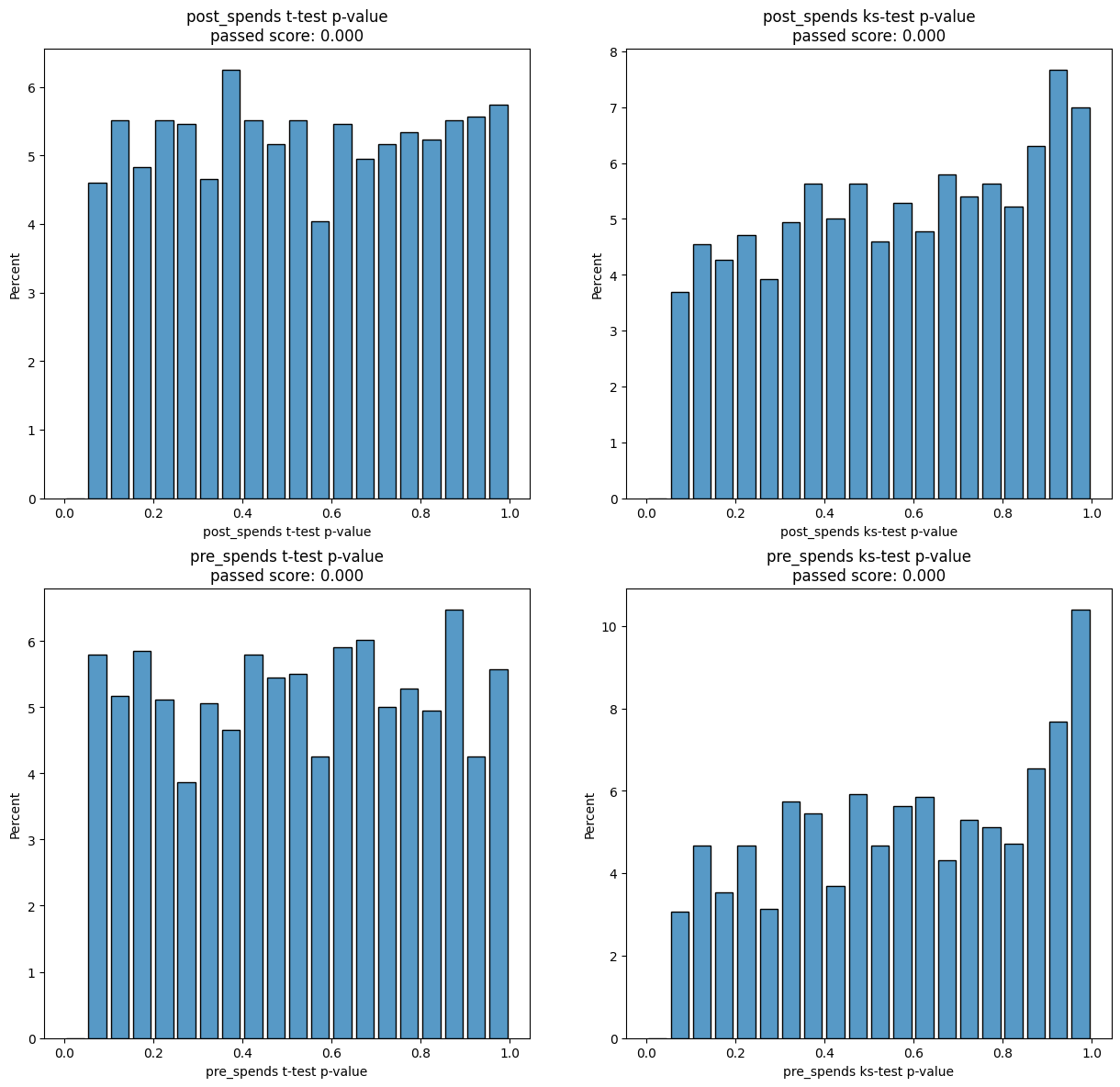

[7]:
show_result(results)
experiments
| random_state | post_spends a mean | post_spends b mean | post_spends ab delta | post_spends ab delta % | post_spends t-test p-value | post_spends ks-test p-value | post_spends t-test passed | post_spends ks-test passed | pre_spends a mean | ... | pre_spends ks-test passed | control % | test % | control size | test size | t-test mean p-value | ks-test mean p-value | t-test passed % | ks-test passed % | mean_tests_score | |
|---|---|---|---|---|---|---|---|---|---|---|---|---|---|---|---|---|---|---|---|---|---|
| 0 | 1 | 452.18 | 452.15 | -0.03 | -0.01 | 0.97 | 0.56 | False | False | 487.33 | ... | False | 50.00 | 50.00 | 5000 | 5000 | 0.59 | 0.49 | 0.00 | 0.00 | 0.52 |
| 1 | 2 | 452.82 | 451.50 | -1.32 | -0.29 | 0.09 | 0.18 | False | False | 487.04 | ... | False | 50.00 | 50.00 | 5000 | 5000 | 0.44 | 0.45 | 0.00 | 0.00 | 0.45 |
| 2 | 4 | 452.41 | 451.92 | -0.50 | -0.11 | 0.53 | 0.06 | False | False | 487.20 | ... | False | 50.00 | 50.00 | 5000 | 5000 | 0.56 | 0.36 | 0.00 | 0.00 | 0.43 |
| 3 | 5 | 452.64 | 451.69 | -0.96 | -0.21 | 0.23 | 0.41 | False | False | 486.90 | ... | False | 50.00 | 50.00 | 5000 | 5000 | 0.26 | 0.40 | 0.00 | 0.00 | 0.35 |
| 4 | 6 | 452.70 | 451.63 | -1.07 | -0.24 | 0.17 | 0.53 | False | False | 487.31 | ... | False | 50.00 | 50.00 | 5000 | 5000 | 0.21 | 0.35 | 0.00 | 0.00 | 0.30 |
| ... | ... | ... | ... | ... | ... | ... | ... | ... | ... | ... | ... | ... | ... | ... | ... | ... | ... | ... | ... | ... | ... |
| 1755 | 1993 | 452.29 | 452.04 | -0.24 | -0.05 | 0.76 | 0.95 | False | False | 486.96 | ... | False | 50.00 | 50.00 | 5000 | 5000 | 0.61 | 0.71 | 0.00 | 0.00 | 0.68 |
| 1756 | 1994 | 452.56 | 451.77 | -0.78 | -0.17 | 0.32 | 0.11 | False | False | 487.12 | ... | False | 50.00 | 50.00 | 5000 | 5000 | 0.61 | 0.21 | 0.00 | 0.00 | 0.34 |
| 1757 | 1995 | 452.30 | 452.03 | -0.26 | -0.06 | 0.74 | 0.91 | False | False | 486.94 | ... | False | 50.00 | 50.00 | 5000 | 5000 | 0.57 | 0.89 | 0.00 | 0.00 | 0.79 |
| 1758 | 1996 | 451.89 | 452.44 | 0.55 | 0.12 | 0.48 | 0.78 | False | False | 487.30 | ... | False | 50.00 | 50.00 | 5000 | 5000 | 0.38 | 0.86 | 0.00 | 0.00 | 0.70 |
| 1759 | 1997 | 452.52 | 451.81 | -0.70 | -0.16 | 0.37 | 0.10 | False | False | 487.10 | ... | False | 50.00 | 50.00 | 5000 | 5000 | 0.66 | 0.40 | 0.00 | 0.00 | 0.49 |
1760 rows × 26 columns
aa_score
| t-test passed score | ks-test passed score | t-test aa passed | ks-test aa passed | |
|---|---|---|---|---|
| post_spends | 0.00 | 0.00 | 0.00 | 0.00 |
| pre_spends | 0.00 | 0.00 | 0.00 | 0.00 |
| mean | 0.00 | 0.00 | 0.00 | 0.00 |
split
| user_id | signup_month | treat | pre_spends | post_spends | age | gender | industry | group | |
|---|---|---|---|---|---|---|---|---|---|
| 0 | 0 | 0 | 0 | 488.00 | 414.44 | NaN | M | E-commerce | test |
| 1 | 1 | 8 | 1 | 512.50 | 462.22 | 26.00 | NaN | E-commerce | test |
| 2 | 4 | 1 | 1 | 543.00 | 514.56 | 18.00 | F | E-commerce | test |
| 3 | 5 | 6 | 1 | 486.50 | 486.56 | 44.00 | M | E-commerce | test |
| 4 | 8 | 4 | 1 | 465.50 | 506.00 | 66.00 | M | Logistics | test |
| ... | ... | ... | ... | ... | ... | ... | ... | ... | ... |
| 9995 | 9990 | 0 | 0 | 490.00 | 426.00 | NaN | M | Logistics | control |
| 9996 | 9992 | 0 | 0 | 491.50 | 424.00 | 29.00 | M | E-commerce | control |
| 9997 | 9996 | 0 | 0 | 500.50 | 430.89 | 26.00 | F | Logistics | control |
| 9998 | 9997 | 3 | 1 | 473.00 | 534.11 | 22.00 | F | E-commerce | control |
| 9999 | 9998 | 2 | 1 | 495.00 | 523.22 | 67.00 | F | E-commerce | control |
10000 rows × 9 columns
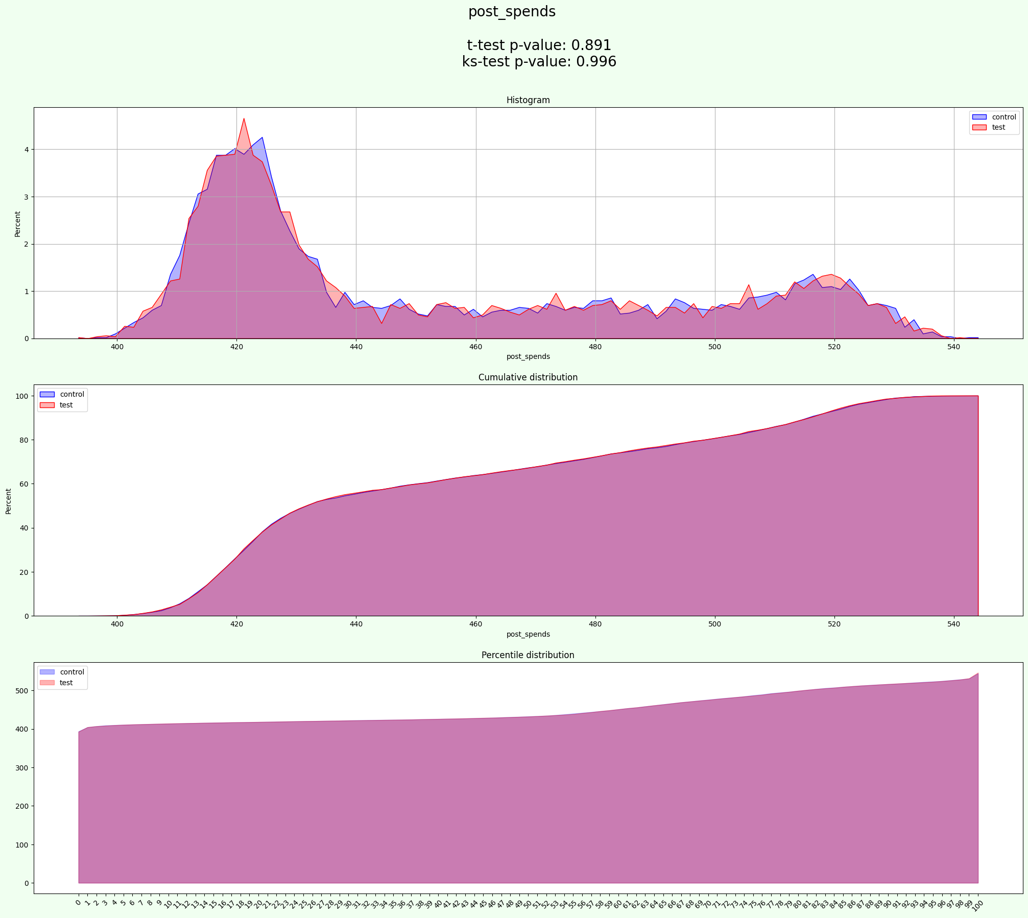
best_experiment_stat
| a mean | b mean | ab delta | ab delta % | t-test p-value | ks-test p-value | t-test passed | ks-test passed | |
|---|---|---|---|---|---|---|---|---|
| post_spends | 452.22 | 452.11 | -0.11 | -0.02 | 0.89 | 1.00 | False | False |
| pre_spends | 487.09 | 487.10 | 0.00 | 0.00 | 0.99 | 1.00 | False | False |
split_stat
control %              50.00
test %                 50.00
control size            5000
test size               5000
t-test mean p-value     0.94
ks-test mean p-value    1.00
t-test passed %         0.00
ks-test passed %        0.00
mean_tests_score        0.98
Name: 60, dtype: object
resume
| aa test passed | split is uniform | |
|---|---|---|
| post_spends | not OK | OK |
| pre_spends | not OK | OK |
[8]:
results.keys()
[8]:
dict_keys(['experiments', 'aa_score', 'split', 'best_experiment_stat', 'split_stat', 'resume'])
results is a dictionary with dataframes as values.
‘split’ - result of separation, column ‘group’ contains values ‘test’ and ‘control’
‘resume’ - summary of all results
‘aa_score’ - score of T-test and Kolmogorov-Smirnov test
‘experiments’ - is a table of results of experiments, which includes
means of all targets in a and b samples,
p_values of Student t-test and test Kolmogorova-Smirnova,
and results of tests (did data on the random_state passes the uniform test)
‘best_experiment_stat’ - like previous point but only for the best experiment
‘split_stat’ - metrics and statistics tests for result of split
[9]:
results['aa_score']
[9]:
| t-test passed score | ks-test passed score | t-test aa passed | ks-test aa passed | |
|---|---|---|---|---|
| post_spends | 0.00 | 0.00 | 0.00 | 0.00 |
| pre_spends | 0.00 | 0.00 | 0.00 | 0.00 |
| mean | 0.00 | 0.00 | 0.00 | 0.00 |
[10]:
results['resume']
[10]:
| aa test passed | split is uniform | |
|---|---|---|
| post_spends | not OK | OK |
| pre_spends | not OK | OK |
2.2 Single experiment
To get stable results lets fix random_state
[11]:
random_state = 11
To perform single experiment you can use sampling_metrics()
[12]:
experiment = AATest(info_cols=info_cols, target_fields=target)
metrics, dict_of_datas = experiment.sampling_metrics(data=data, random_state=random_state).values()
The results contains the same info as in multisampling, but on one experiment
[13]:
metrics
[13]:
{'random_state': 11,
 'post_spends a mean': 451.8546,
 'post_spends b mean': 452.4745111111112,
 'post_spends ab delta': 0.6199111111112074,
 'post_spends ab delta %': 0.13700464797208323,
 'post_spends t-test p-value': 0.43154056610193947,
 'post_spends ks-test p-value': 0.95721723072851,
 'post_spends t-test passed': False,
 'post_spends ks-test passed': False,
 'pre_spends a mean': 487.2131,
 'pre_spends b mean': 486.9744,
 'pre_spends ab delta': -0.23869999999999436,
 'pre_spends ab delta %': -0.04901695037766718,
 'pre_spends t-test p-value': 0.5271083329122467,
 'pre_spends ks-test p-value': 0.14861030130677552,
 'pre_spends t-test passed': False,
 'pre_spends ks-test passed': False,
 'control %': 50.0,
 'test %': 50.0,
 'control size': 5000,
 'test size': 5000,
 't-test mean p-value': 0.4793244495070931,
 'ks-test mean p-value': 0.5529137660176427,
 't-test passed %': 0.0,
 'ks-test passed %': 0.0,
 'mean_tests_score': 0.5283839938474595}
[14]:
dict_of_datas[random_state]
[14]:
| user_id | signup_month | treat | pre_spends | post_spends | age | gender | industry | group | |
|---|---|---|---|---|---|---|---|---|---|
| 0 | 1 | 8 | 1 | 512.50 | 462.22 | 26.00 | NaN | E-commerce | test |
| 1 | 2 | 7 | 1 | 483.00 | 479.44 | 25.00 | M | Logistics | test |
| 2 | 5 | 6 | 1 | 486.50 | 486.56 | 44.00 | M | E-commerce | test |
| 3 | 6 | 11 | 1 | 483.50 | 433.89 | 28.00 | F | Logistics | test |
| 4 | 11 | 4 | 1 | 498.50 | 516.89 | 58.00 | NaN | E-commerce | test |
| ... | ... | ... | ... | ... | ... | ... | ... | ... | ... |
| 9995 | 9986 | 0 | 0 | 494.00 | 432.11 | 39.00 | M | Logistics | control |
| 9996 | 9989 | 6 | 1 | 466.50 | 487.44 | 19.00 | F | E-commerce | control |
| 9997 | 9991 | 0 | 0 | 482.50 | 421.89 | 43.00 | NaN | Logistics | control |
| 9998 | 9995 | 10 | 1 | 538.50 | 450.44 | 42.00 | M | Logistics | control |
| 9999 | 9998 | 2 | 1 | 495.00 | 523.22 | 67.00 | F | E-commerce | control |
10000 rows × 9 columns
[15]:
results = experiment.experiment_result_transform(pd.Series(metrics))
[16]:
results.keys()
[16]:
dict_keys(['best_experiment_stat', 'best_split_stat'])
[17]:
results['best_experiment_stat']
[17]:
| a mean | b mean | ab delta | ab delta % | t-test p-value | ks-test p-value | t-test passed | ks-test passed | |
|---|---|---|---|---|---|---|---|---|
| post_spends | 451.85 | 452.47 | 0.62 | 0.14 | 0.43 | 0.96 | False | False |
| pre_spends | 487.21 | 486.97 | -0.24 | -0.05 | 0.53 | 0.15 | False | False |
[18]:
results['best_split_stat']
[18]:
control %              50.00
test %                 50.00
control size            5000
test size               5000
t-test mean p-value     0.48
ks-test mean p-value    0.55
t-test passed %         0.00
ks-test passed %        0.00
mean_tests_score        0.53
dtype: object
2.3 AA-test with grouping
To perform experiment that separates samples by groups group_col can be used
[19]:
info_cols = ['user_id', 'signup_month']
target = ['post_spends', 'pre_spends']
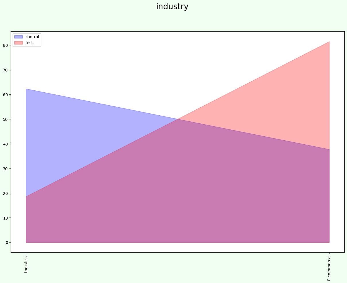
group_cols = 'industry'
[20]:
experiment = AATest(info_cols=info_cols, target_fields=target, group_cols=group_cols)
[21]:
results = experiment.process(data=data, iterations=2000)
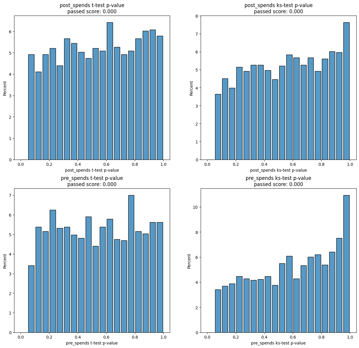

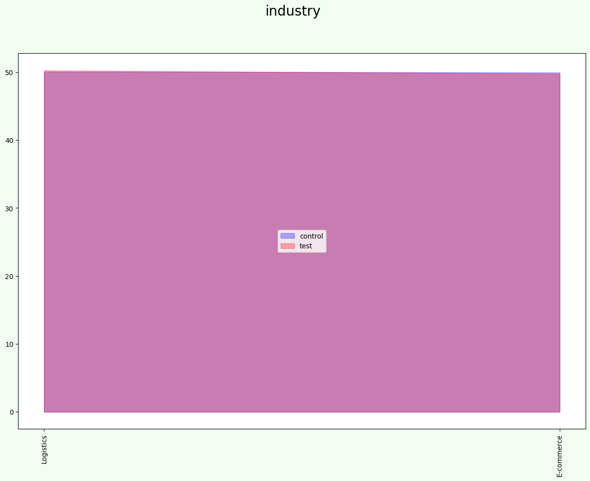
The result is in the same format as without groups
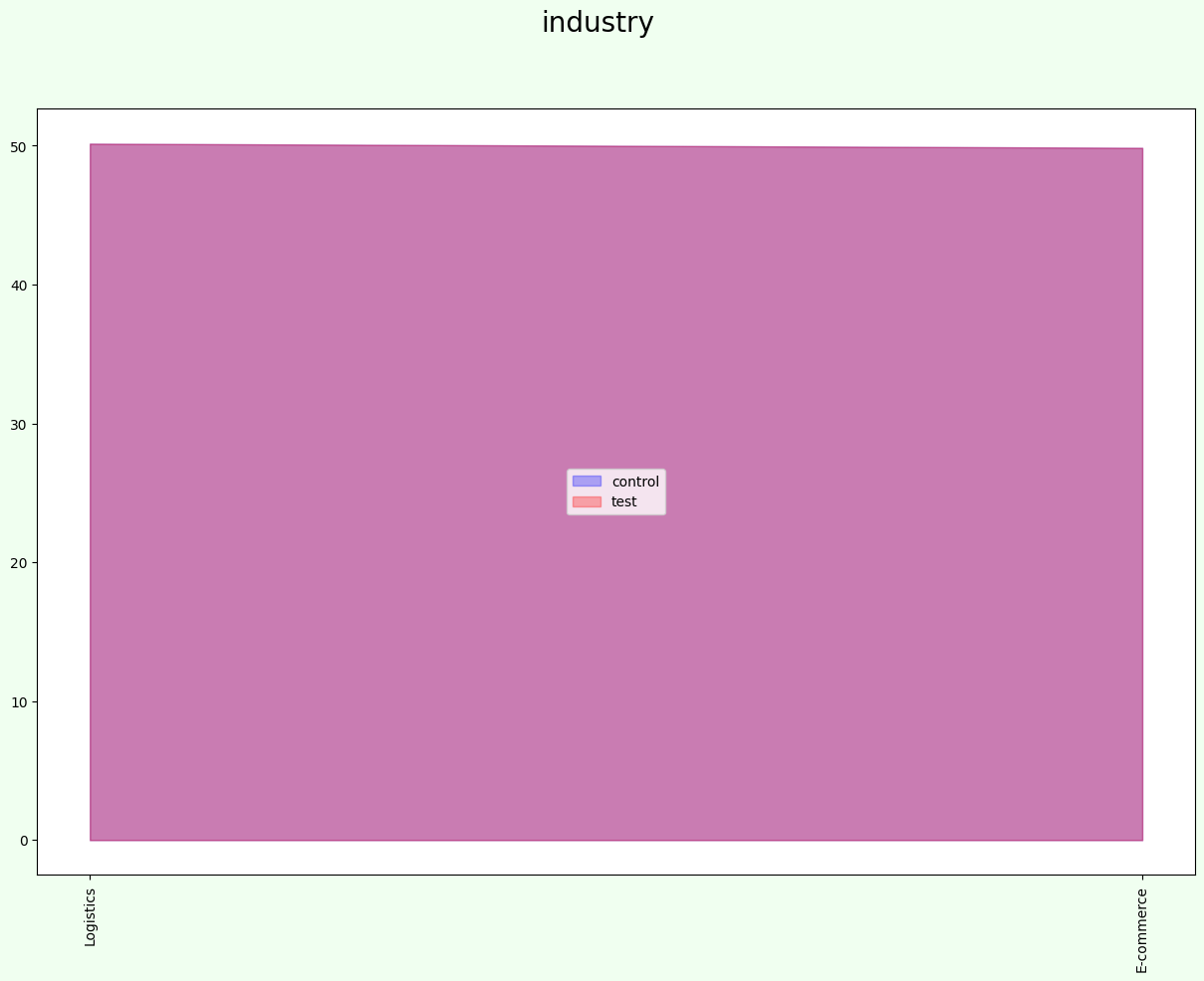
In this regime groups equally divided on each sample (test and control):
[22]:
results['split']['industry'].value_counts(normalize=True) * 100
[22]:
industry
Logistics    50.15
E-commerce   49.85
Name: proportion, dtype: float64
[23]:
results['split'].groupby(['industry', 'group'])[['user_id']].count()
[23]:
| user_id | ||
|---|---|---|
| industry | group | |
| E-commerce | control | 2493 |
| test | 2492 | |
| Logistics | control | 2508 |
| test | 2507 |
[24]:
show_result(results)
experiments
| random_state | post_spends a mean | post_spends b mean | post_spends ab delta | post_spends ab delta % | post_spends t-test p-value | post_spends ks-test p-value | post_spends t-test passed | post_spends ks-test passed | pre_spends a mean | ... | pre_spends ks-test passed | control % | test % | control size | test size | t-test mean p-value | ks-test mean p-value | t-test passed % | ks-test passed % | mean_tests_score | |
|---|---|---|---|---|---|---|---|---|---|---|---|---|---|---|---|---|---|---|---|---|---|
| 0 | 0 | 451.53 | 452.80 | 1.27 | 0.28 | 0.11 | 0.19 | False | False | 487.00 | ... | False | 50.01 | 49.99 | 5001 | 4999 | 0.36 | 0.52 | 0.00 | 0.00 | 0.47 |
| 1 | 2 | 452.53 | 451.80 | -0.73 | -0.16 | 0.35 | 0.83 | False | False | 487.19 | ... | False | 50.01 | 49.99 | 5001 | 4999 | 0.47 | 0.92 | 0.00 | 0.00 | 0.77 |
| 2 | 3 | 452.10 | 452.23 | 0.13 | 0.03 | 0.87 | 0.85 | False | False | 487.11 | ... | False | 50.01 | 49.99 | 5001 | 4999 | 0.90 | 0.93 | 0.00 | 0.00 | 0.92 |
| 3 | 4 | 452.18 | 452.15 | -0.03 | -0.01 | 0.97 | 0.30 | False | False | 487.20 | ... | False | 50.01 | 49.99 | 5001 | 4999 | 0.77 | 0.47 | 0.00 | 0.00 | 0.57 |
| 4 | 7 | 452.38 | 451.95 | -0.42 | -0.09 | 0.59 | 0.40 | False | False | 487.20 | ... | False | 50.01 | 49.99 | 5001 | 4999 | 0.58 | 0.50 | 0.00 | 0.00 | 0.53 |
| ... | ... | ... | ... | ... | ... | ... | ... | ... | ... | ... | ... | ... | ... | ... | ... | ... | ... | ... | ... | ... | ... |
| 1723 | 1995 | 452.70 | 451.63 | -1.07 | -0.24 | 0.18 | 0.14 | False | False | 487.40 | ... | False | 50.01 | 49.99 | 5001 | 4999 | 0.14 | 0.16 | 0.00 | 0.00 | 0.16 |
| 1724 | 1996 | 452.36 | 451.96 | -0.40 | -0.09 | 0.61 | 0.81 | False | False | 487.08 | ... | False | 50.01 | 49.99 | 5001 | 4999 | 0.78 | 0.69 | 0.00 | 0.00 | 0.72 |
| 1725 | 1997 | 452.08 | 452.25 | 0.18 | 0.04 | 0.82 | 0.59 | False | False | 487.04 | ... | False | 50.01 | 49.99 | 5001 | 4999 | 0.79 | 0.66 | 0.00 | 0.00 | 0.70 |
| 1726 | 1998 | 451.96 | 452.36 | 0.40 | 0.09 | 0.61 | 0.44 | False | False | 486.85 | ... | False | 50.01 | 49.99 | 5001 | 4999 | 0.41 | 0.54 | 0.00 | 0.00 | 0.50 |
| 1727 | 1999 | 452.38 | 451.95 | -0.42 | -0.09 | 0.59 | 0.54 | False | False | 487.21 | ... | False | 50.01 | 49.99 | 5001 | 4999 | 0.57 | 0.62 | 0.00 | 0.00 | 0.60 |
1728 rows × 26 columns
aa_score
| t-test passed score | ks-test passed score | t-test aa passed | ks-test aa passed | |
|---|---|---|---|---|
| post_spends | 0.00 | 0.00 | 0.00 | 0.00 |
| pre_spends | 0.00 | 0.00 | 0.00 | 0.00 |
| mean | 0.00 | 0.00 | 0.00 | 0.00 |
split
| user_id | signup_month | treat | pre_spends | post_spends | age | gender | industry | group | |
|---|---|---|---|---|---|---|---|---|---|
| 0 | 0 | 0 | 0 | 488.00 | 414.44 | NaN | M | E-commerce | test |
| 1 | 2 | 7 | 1 | 483.00 | 479.44 | 25.00 | M | Logistics | test |
| 2 | 4 | 1 | 1 | 543.00 | 514.56 | 18.00 | F | E-commerce | test |
| 3 | 5 | 6 | 1 | 486.50 | 486.56 | 44.00 | M | E-commerce | test |
| 4 | 7 | 11 | 1 | 496.00 | 432.89 | 57.00 | M | E-commerce | test |
| ... | ... | ... | ... | ... | ... | ... | ... | ... | ... |
| 9995 | 9983 | 0 | 0 | 494.50 | 428.33 | 31.00 | F | Logistics | control |
| 9996 | 9984 | 0 | 0 | 460.00 | 417.11 | 56.00 | M | Logistics | control |
| 9997 | 9985 | 0 | 0 | 484.00 | 411.33 | 52.00 | M | E-commerce | control |
| 9998 | 9991 | 0 | 0 | 482.50 | 421.89 | 43.00 | NaN | Logistics | control |
| 9999 | 9994 | 0 | 0 | 486.00 | 423.78 | 69.00 | F | Logistics | control |
10000 rows × 9 columns
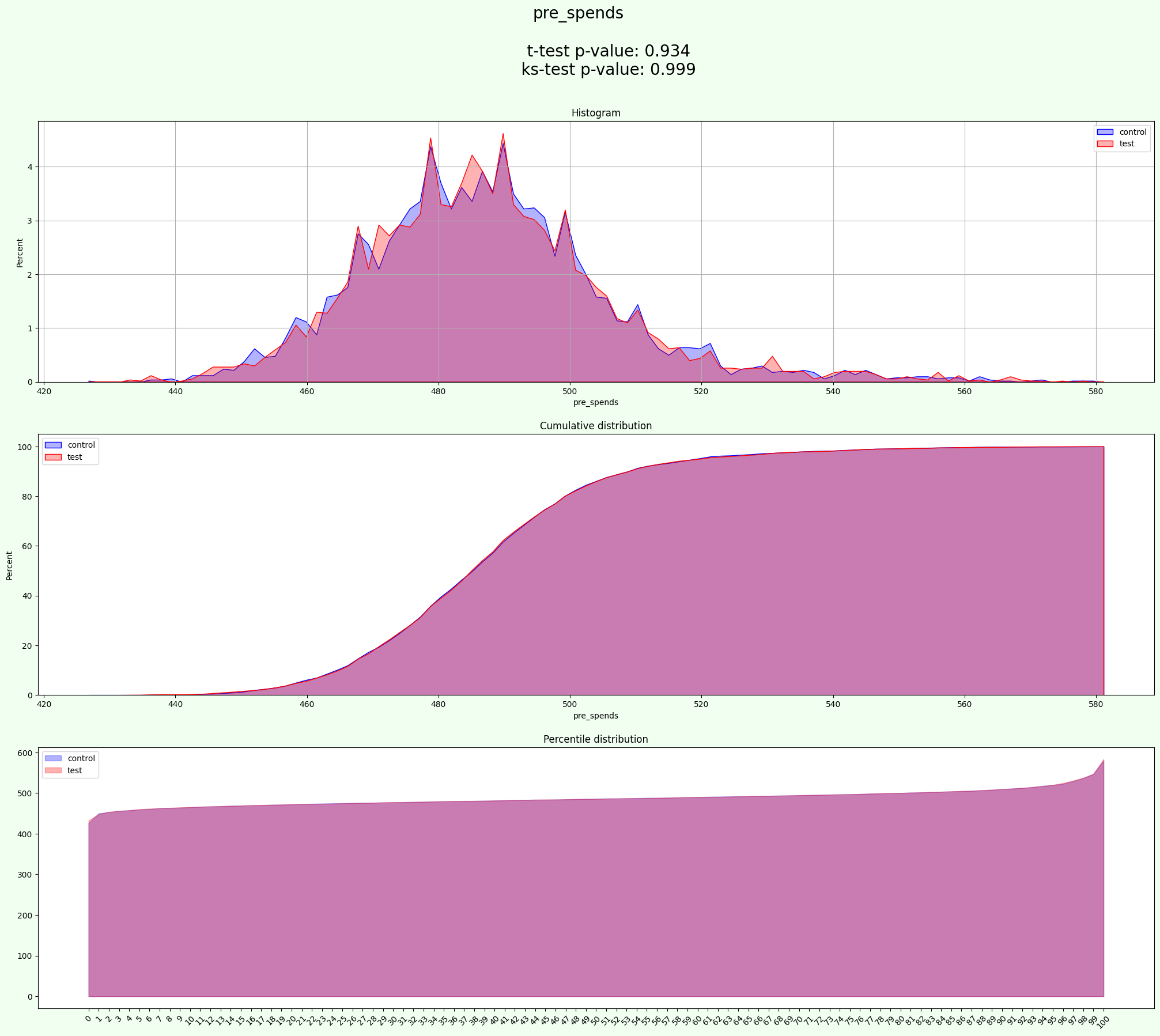
best_experiment_stat
| a mean | b mean | ab delta | ab delta % | t-test p-value | ks-test p-value | t-test passed | ks-test passed | |
|---|---|---|---|---|---|---|---|---|
| post_spends | 452.18 | 452.15 | -0.03 | -0.01 | 0.97 | 0.99 | False | False |
| pre_spends | 487.08 | 487.11 | 0.03 | 0.01 | 0.93 | 1.00 | False | False |
split_stat
control %              50.01
test %                 49.99
control size            5001
test size               4999
t-test mean p-value     0.95
ks-test mean p-value    0.99
t-test passed %         0.00
ks-test passed %        0.00
mean_tests_score        0.98
Name: 1395, dtype: object
resume
| aa test passed | split is uniform | |
|---|---|---|
| post_spends | not OK | OK |
| pre_spends | not OK | OK |
2.4 AA with optimize group
If you have many columns for grouping and don’t know which colun or columns will make best result, you can use parametr ``optimize_group=True``. AA-Test will choose optimal number and names of group columns.
You can use columns_labeling to automatically name columns as target and group.
[25]:
experiment.columns_labeling(data)
[25]:
{'target_field': ['treat', 'pre_spends', 'post_spends', 'age'],
 'group_col': ['gender', 'industry']}
[26]:
results = experiment.process(data=data, optimize_groups=True, iterations=2000)


[27]:
experiment.group_cols
[27]:
['industry']
[28]:
show_result(results)
experiments
| random_state | post_spends a mean | post_spends b mean | post_spends ab delta | post_spends ab delta % | post_spends t-test p-value | post_spends ks-test p-value | post_spends t-test passed | post_spends ks-test passed | pre_spends a mean | ... | pre_spends ks-test passed | control % | test % | control size | test size | t-test mean p-value | ks-test mean p-value | t-test passed % | ks-test passed % | mean_tests_score | |
|---|---|---|---|---|---|---|---|---|---|---|---|---|---|---|---|---|---|---|---|---|---|
| 0 | 0 | 452.60 | 451.72 | -0.88 | -0.19 | 0.26 | 0.48 | False | False | 487.38 | ... | True | 50.00 | 50.00 | 5000 | 5000 | 0.20 | 0.25 | 0.00 | 50.00 | 0.23 |
| 1 | 1 | 452.18 | 452.15 | -0.03 | -0.01 | 0.97 | 0.56 | False | False | 487.33 | ... | False | 50.00 | 50.00 | 5000 | 5000 | 0.59 | 0.49 | 0.00 | 0.00 | 0.52 |
| 2 | 2 | 452.82 | 451.50 | -1.32 | -0.29 | 0.09 | 0.18 | False | False | 487.04 | ... | False | 50.00 | 50.00 | 5000 | 5000 | 0.44 | 0.45 | 0.00 | 0.00 | 0.45 |
| 3 | 3 | 451.25 | 453.08 | 1.83 | 0.40 | 0.02 | 0.08 | True | False | 486.67 | ... | False | 50.00 | 50.00 | 5000 | 5000 | 0.02 | 0.13 | 100.00 | 0.00 | 0.09 |
| 4 | 4 | 452.41 | 451.92 | -0.50 | -0.11 | 0.53 | 0.06 | False | False | 487.20 | ... | False | 50.00 | 50.00 | 5000 | 5000 | 0.56 | 0.36 | 0.00 | 0.00 | 0.43 |
| ... | ... | ... | ... | ... | ... | ... | ... | ... | ... | ... | ... | ... | ... | ... | ... | ... | ... | ... | ... | ... | ... |
| 1995 | 1995 | 452.30 | 452.03 | -0.26 | -0.06 | 0.74 | 0.91 | False | False | 486.94 | ... | False | 50.00 | 50.00 | 5000 | 5000 | 0.57 | 0.89 | 0.00 | 0.00 | 0.79 |
| 1996 | 1996 | 451.89 | 452.44 | 0.55 | 0.12 | 0.48 | 0.78 | False | False | 487.30 | ... | False | 50.00 | 50.00 | 5000 | 5000 | 0.38 | 0.86 | 0.00 | 0.00 | 0.70 |
| 1997 | 1997 | 452.52 | 451.81 | -0.70 | -0.16 | 0.37 | 0.10 | False | False | 487.10 | ... | False | 50.00 | 50.00 | 5000 | 5000 | 0.66 | 0.40 | 0.00 | 0.00 | 0.49 |
| 1998 | 1998 | 452.27 | 452.06 | -0.21 | -0.05 | 0.79 | 0.86 | False | False | 486.73 | ... | True | 50.00 | 50.00 | 5000 | 5000 | 0.42 | 0.45 | 0.00 | 50.00 | 0.44 |
| 1999 | 1999 | 451.47 | 452.86 | 1.38 | 0.31 | 0.08 | 0.02 | False | True | 486.75 | ... | False | 50.00 | 50.00 | 5000 | 5000 | 0.07 | 0.36 | 0.00 | 50.00 | 0.26 |
2000 rows × 26 columns
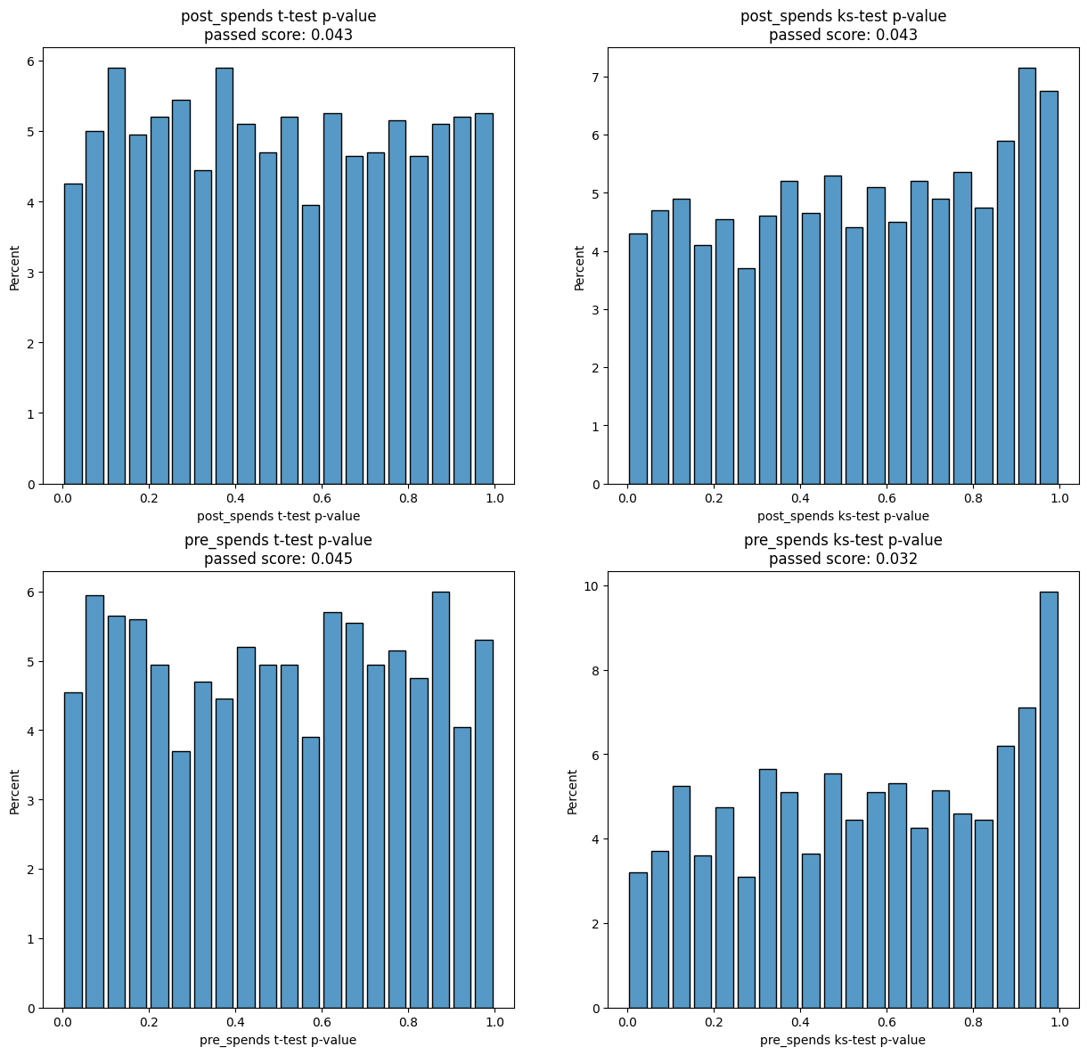
aa_score
| t-test passed score | ks-test passed score | t-test aa passed | ks-test aa passed | |
|---|---|---|---|---|
| post_spends | 0.04 | 0.04 | 1.00 | 1.00 |
| pre_spends | 0.05 | 0.03 | 1.00 | 0.00 |
| mean | 0.04 | 0.04 | 1.00 | 0.50 |
split
| user_id | signup_month | treat | pre_spends | post_spends | age | gender | industry | group | |
|---|---|---|---|---|---|---|---|---|---|
| 0 | 0 | 0 | 0 | 488.00 | 414.44 | NaN | M | E-commerce | test |
| 1 | 1 | 8 | 1 | 512.50 | 462.22 | 26.00 | NaN | E-commerce | test |
| 2 | 4 | 1 | 1 | 543.00 | 514.56 | 18.00 | F | E-commerce | test |
| 3 | 5 | 6 | 1 | 486.50 | 486.56 | 44.00 | M | E-commerce | test |
| 4 | 8 | 4 | 1 | 465.50 | 506.00 | 66.00 | M | Logistics | test |
| ... | ... | ... | ... | ... | ... | ... | ... | ... | ... |
| 9995 | 9990 | 0 | 0 | 490.00 | 426.00 | NaN | M | Logistics | control |
| 9996 | 9992 | 0 | 0 | 491.50 | 424.00 | 29.00 | M | E-commerce | control |
| 9997 | 9996 | 0 | 0 | 500.50 | 430.89 | 26.00 | F | Logistics | control |
| 9998 | 9997 | 3 | 1 | 473.00 | 534.11 | 22.00 | F | E-commerce | control |
| 9999 | 9998 | 2 | 1 | 495.00 | 523.22 | 67.00 | F | E-commerce | control |
10000 rows × 9 columns
best_experiment_stat
| a mean | b mean | ab delta | ab delta % | t-test p-value | ks-test p-value | t-test passed | ks-test passed | |
|---|---|---|---|---|---|---|---|---|
| post_spends | 452.22 | 452.11 | -0.11 | -0.02 | 0.89 | 1.00 | False | False |
| pre_spends | 487.09 | 487.10 | 0.00 | 0.00 | 0.99 | 1.00 | False | False |
split_stat
control %              50.00
test %                 50.00
control size            5000
test size               5000
t-test mean p-value     0.94
ks-test mean p-value    1.00
t-test passed %         0.00
ks-test passed %        0.00
mean_tests_score        0.98
Name: 69, dtype: object
resume
| aa test passed | split is uniform | |
|---|---|---|
| post_spends | OK | OK |
| pre_spends | OK | OK |
2.5 AA test with quantization
If you want make one column as parameter for quantization, you may use ``quant_field``.
[29]:
info_cols = ['user_id', 'signup_month']
target = ['post_spends', 'pre_spends']

group_cols = 'industry'
quant_field = 'gender'
[30]:
experiment = AATest(info_cols=info_cols, target_fields=target, group_cols=group_cols, quant_field=quant_field)
[31]:
result = experiment.process(data=data, iterations=2000)


[32]:
result['split'].groupby(['gender', 'industry', 'group'])['user_id'].count()
[32]:
gender  industry    group
F       E-commerce  test       2261
        Logistics   control    2305
M       E-commerce  control    2240
        Logistics   control    2194
Name: user_id, dtype: int64
[33]:
show_result(result)
experiments
| random_state | post_spends a mean | post_spends b mean | post_spends ab delta | post_spends ab delta % | post_spends t-test p-value | post_spends ks-test p-value | post_spends t-test passed | post_spends ks-test passed | pre_spends a mean | ... | pre_spends ks-test passed | control % | test % | control size | test size | t-test mean p-value | ks-test mean p-value | t-test passed % | ks-test passed % | mean_tests_score | |
|---|---|---|---|---|---|---|---|---|---|---|---|---|---|---|---|---|---|---|---|---|---|
| 0 | 0 | 452.05 | 452.46 | 0.41 | 0.09 | 0.64 | 0.91 | False | False | 486.90 | ... | False | 72.23 | 27.77 | 7223 | 2777 | 0.37 | 0.62 | 0.00 | 0.00 | 0.53 |
| 1 | 2 | 452.05 | 452.46 | 0.41 | 0.09 | 0.64 | 0.91 | False | False | 486.90 | ... | False | 72.23 | 27.77 | 7223 | 2777 | 0.37 | 0.62 | 0.00 | 0.00 | 0.53 |
| 2 | 7 | 452.05 | 452.46 | 0.41 | 0.09 | 0.64 | 0.91 | False | False | 486.90 | ... | False | 72.23 | 27.77 | 7223 | 2777 | 0.37 | 0.62 | 0.00 | 0.00 | 0.53 |
| 3 | 8 | 452.05 | 452.46 | 0.41 | 0.09 | 0.64 | 0.91 | False | False | 486.90 | ... | False | 72.23 | 27.77 | 7223 | 2777 | 0.37 | 0.62 | 0.00 | 0.00 | 0.53 |
| 4 | 15 | 452.05 | 452.46 | 0.41 | 0.09 | 0.64 | 0.91 | False | False | 486.90 | ... | False | 72.23 | 27.77 | 7223 | 2777 | 0.37 | 0.62 | 0.00 | 0.00 | 0.53 |
| ... | ... | ... | ... | ... | ... | ... | ... | ... | ... | ... | ... | ... | ... | ... | ... | ... | ... | ... | ... | ... | ... |
| 643 | 1981 | 452.05 | 452.46 | 0.41 | 0.09 | 0.64 | 0.91 | False | False | 486.90 | ... | False | 72.23 | 27.77 | 7223 | 2777 | 0.37 | 0.62 | 0.00 | 0.00 | 0.53 |
| 644 | 1982 | 452.05 | 452.46 | 0.41 | 0.09 | 0.64 | 0.91 | False | False | 486.90 | ... | False | 72.23 | 27.77 | 7223 | 2777 | 0.37 | 0.62 | 0.00 | 0.00 | 0.53 |
| 645 | 1984 | 452.05 | 452.46 | 0.41 | 0.09 | 0.64 | 0.91 | False | False | 486.90 | ... | False | 72.23 | 27.77 | 7223 | 2777 | 0.37 | 0.62 | 0.00 | 0.00 | 0.53 |
| 646 | 1988 | 452.05 | 452.46 | 0.41 | 0.09 | 0.64 | 0.91 | False | False | 486.90 | ... | False | 72.23 | 27.77 | 7223 | 2777 | 0.37 | 0.62 | 0.00 | 0.00 | 0.53 |
| 647 | 1998 | 452.05 | 452.46 | 0.41 | 0.09 | 0.64 | 0.91 | False | False | 486.90 | ... | False | 72.23 | 27.77 | 7223 | 2777 | 0.37 | 0.62 | 0.00 | 0.00 | 0.53 |
648 rows × 26 columns
aa_score
| t-test passed score | ks-test passed score | t-test aa passed | ks-test aa passed | |
|---|---|---|---|---|
| post_spends | 0.00 | 0.00 | 0.00 | 0.00 |
| pre_spends | 0.00 | 0.00 | 0.00 | 0.00 |
| mean | 0.00 | 0.00 | 0.00 | 0.00 |
split
| user_id | signup_month | treat | pre_spends | post_spends | age | gender | industry | group | |
|---|---|---|---|---|---|---|---|---|---|
| 0 | 8193 | 0 | 0 | 494.50 | 427.11 | 40.00 | F | E-commerce | test |
| 1 | 8195 | 0 | 0 | 494.00 | 416.22 | 41.00 | F | E-commerce | test |
| 2 | 4 | 1 | 1 | 543.00 | 514.56 | 18.00 | F | E-commerce | test |
| 3 | 8203 | 0 | 0 | 472.50 | 412.67 | 52.00 | F | E-commerce | test |
| 4 | 8205 | 0 | 0 | 460.00 | 408.22 | 66.00 | F | E-commerce | test |
| ... | ... | ... | ... | ... | ... | ... | ... | ... | ... |
| 9995 | 9990 | 0 | 0 | 490.00 | 426.00 | NaN | M | Logistics | control |
| 9996 | 9992 | 0 | 0 | 491.50 | 424.00 | 29.00 | M | E-commerce | control |
| 9997 | 9994 | 0 | 0 | 486.00 | 423.78 | 69.00 | F | Logistics | control |
| 9998 | 9995 | 10 | 1 | 538.50 | 450.44 | 42.00 | M | Logistics | control |
| 9999 | 9996 | 0 | 0 | 500.50 | 430.89 | 26.00 | F | Logistics | control |
10000 rows × 9 columns
best_experiment_stat
| a mean | b mean | ab delta | ab delta % | t-test p-value | ks-test p-value | t-test passed | ks-test passed | |
|---|---|---|---|---|---|---|---|---|
| post_spends | 452.05 | 452.46 | 0.41 | 0.09 | 0.64 | 0.91 | False | False |
| pre_spends | 486.90 | 487.60 | 0.71 | 0.15 | 0.09 | 0.32 | False | False |
split_stat
control %              72.23
test %                 27.77
control size            7223
test size               2777
t-test mean p-value     0.37
ks-test mean p-value    0.62
t-test passed %         0.00
ks-test passed %        0.00
mean_tests_score        0.53
Name: 0, dtype: object
resume
| aa test passed | split is uniform | |
|---|---|---|
| post_spends | not OK | OK |
| pre_spends | not OK | OK |
2.6 Unbalanced AA test
If you want to perform AA test with unbalanced groups, you can use parametr ``test_size`` to define sizes of test group and control group
[34]:
info_cols = ['user_id', 'signup_month']
target = ['post_spends', 'pre_spends']

group_cols = 'industry'
[35]:
experiment = AATest(info_cols=info_cols, target_fields=target, group_cols=group_cols)
[36]:
result = experiment.process(data=data, test_size=0.3, iterations=2000)


[37]:
result['split']['group'].value_counts(normalize=True)
[37]:
group
control   0.70
test      0.30
Name: proportion, dtype: float64
[38]:
show_result(result)
experiments
| random_state | post_spends a mean | post_spends b mean | post_spends ab delta | post_spends ab delta % | post_spends t-test p-value | post_spends ks-test p-value | post_spends t-test passed | post_spends ks-test passed | pre_spends a mean | ... | pre_spends ks-test passed | control % | test % | control size | test size | t-test mean p-value | ks-test mean p-value | t-test passed % | ks-test passed % | mean_tests_score | |
|---|---|---|---|---|---|---|---|---|---|---|---|---|---|---|---|---|---|---|---|---|---|
| 0 | 1 | 451.99 | 452.57 | 0.57 | 0.13 | 0.50 | 0.76 | False | False | 487.11 | ... | False | 70.01 | 29.99 | 7001 | 2999 | 0.69 | 0.66 | 0.00 | 0.00 | 0.67 |
| 1 | 2 | 452.16 | 452.17 | 0.01 | 0.00 | 0.99 | 0.64 | False | False | 487.00 | ... | False | 70.01 | 29.99 | 7001 | 2999 | 0.73 | 0.72 | 0.00 | 0.00 | 0.72 |
| 2 | 3 | 452.22 | 452.03 | -0.20 | -0.04 | 0.82 | 0.59 | False | False | 487.18 | ... | False | 70.01 | 29.99 | 7001 | 2999 | 0.66 | 0.48 | 0.00 | 0.00 | 0.54 |
| 3 | 4 | 451.90 | 452.78 | 0.88 | 0.19 | 0.31 | 0.24 | False | False | 487.13 | ... | False | 70.01 | 29.99 | 7001 | 2999 | 0.54 | 0.60 | 0.00 | 0.00 | 0.58 |
| 4 | 5 | 452.64 | 451.05 | -1.59 | -0.35 | 0.06 | 0.14 | False | False | 487.20 | ... | False | 70.01 | 29.99 | 7001 | 2999 | 0.23 | 0.14 | 0.00 | 0.00 | 0.17 |
| ... | ... | ... | ... | ... | ... | ... | ... | ... | ... | ... | ... | ... | ... | ... | ... | ... | ... | ... | ... | ... | ... |
| 1705 | 1995 | 452.12 | 452.28 | 0.16 | 0.04 | 0.85 | 0.63 | False | False | 487.10 | ... | False | 70.01 | 29.99 | 7001 | 2999 | 0.89 | 0.64 | 0.00 | 0.00 | 0.73 |
| 1706 | 1996 | 452.00 | 452.54 | 0.54 | 0.12 | 0.53 | 0.85 | False | False | 486.94 | ... | False | 70.01 | 29.99 | 7001 | 2999 | 0.37 | 0.72 | 0.00 | 0.00 | 0.60 |
| 1707 | 1997 | 452.29 | 451.88 | -0.40 | -0.09 | 0.64 | 0.60 | False | False | 487.04 | ... | False | 70.01 | 29.99 | 7001 | 2999 | 0.65 | 0.44 | 0.00 | 0.00 | 0.51 |
| 1708 | 1998 | 451.78 | 453.07 | 1.29 | 0.28 | 0.13 | 0.33 | False | False | 487.12 | ... | False | 70.01 | 29.99 | 7001 | 2999 | 0.47 | 0.66 | 0.00 | 0.00 | 0.60 |
| 1709 | 1999 | 452.25 | 451.96 | -0.29 | -0.06 | 0.74 | 0.77 | False | False | 487.17 | ... | False | 70.01 | 29.99 | 7001 | 2999 | 0.64 | 0.71 | 0.00 | 0.00 | 0.69 |
1710 rows × 26 columns
aa_score
| t-test passed score | ks-test passed score | t-test aa passed | ks-test aa passed | |
|---|---|---|---|---|
| post_spends | 0.00 | 0.00 | 0.00 | 0.00 |
| pre_spends | 0.00 | 0.00 | 0.00 | 0.00 |
| mean | 0.00 | 0.00 | 0.00 | 0.00 |
split
| user_id | signup_month | treat | pre_spends | post_spends | age | gender | industry | group | |
|---|---|---|---|---|---|---|---|---|---|
| 0 | 0 | 0 | 0 | 488.00 | 414.44 | NaN | M | E-commerce | test |
| 1 | 8193 | 0 | 0 | 494.50 | 427.11 | 40.00 | F | E-commerce | test |
| 2 | 8192 | 0 | 0 | 487.50 | 436.78 | 20.00 | M | E-commerce | test |
| 3 | 2 | 7 | 1 | 483.00 | 479.44 | 25.00 | M | Logistics | test |
| 4 | 8200 | 5 | 1 | 486.00 | 495.00 | NaN | M | Logistics | test |
| ... | ... | ... | ... | ... | ... | ... | ... | ... | ... |
| 9995 | 9994 | 0 | 0 | 486.00 | 423.78 | 69.00 | F | Logistics | control |
| 9996 | 9995 | 10 | 1 | 538.50 | 450.44 | 42.00 | M | Logistics | control |
| 9997 | 9997 | 3 | 1 | 473.00 | 534.11 | 22.00 | F | E-commerce | control |
| 9998 | 9998 | 2 | 1 | 495.00 | 523.22 | 67.00 | F | E-commerce | control |
| 9999 | 9999 | 7 | 1 | 508.00 | 475.89 | 38.00 | F | E-commerce | control |
10000 rows × 9 columns
best_experiment_stat
| a mean | b mean | ab delta | ab delta % | t-test p-value | ks-test p-value | t-test passed | ks-test passed | |
|---|---|---|---|---|---|---|---|---|
| post_spends | 452.15 | 452.19 | 0.04 | 0.01 | 0.96 | 0.99 | False | False |
| pre_spends | 487.09 | 487.09 | -0.00 | -0.00 | 1.00 | 0.99 | False | False |
split_stat
control %              70.01
test %                 29.99
control size            7001
test size               2999
t-test mean p-value     0.98
ks-test mean p-value    0.99
t-test passed %         0.00
ks-test passed %        0.00
mean_tests_score        0.99
Name: 1472, dtype: object
resume
| aa test passed | split is uniform | |
|---|---|---|
| post_spends | not OK | OK |
| pre_spends | not OK | OK |
MDE
this is the boundary value of the effect, for which it makes sense to introduce some changes.
[39]:
info_cols = ['user_id', 'signup_month']
target = ['post_spends', 'pre_spends']

group_cols = 'industry'
mde_target = 'post_spends'
[40]:
experiment = AATest(info_cols=info_cols, target_fields=target, group_cols=group_cols)
Single experiment of data splitting for MDE calculation.
P.s. [None] is the number of random state. You can change it like sampling_metrics(data, random_state=42) and get result with [42] instead of [None]
[41]:
splitted_data = experiment.sampling_metrics(data)['data_from_experiment'][None]
splitted_data
[41]:
| user_id | signup_month | treat | pre_spends | post_spends | age | gender | industry | group | |
|---|---|---|---|---|---|---|---|---|---|
| 0 | 0 | 0 | 0 | 488.00 | 414.44 | NaN | M | E-commerce | test |
| 1 | 2 | 7 | 1 | 483.00 | 479.44 | 25.00 | M | Logistics | test |
| 2 | 5 | 6 | 1 | 486.50 | 486.56 | 44.00 | M | E-commerce | test |
| 3 | 7 | 11 | 1 | 496.00 | 432.89 | 57.00 | M | E-commerce | test |
| 4 | 9 | 4 | 1 | 470.00 | 512.11 | 54.00 | M | Logistics | test |
| ... | ... | ... | ... | ... | ... | ... | ... | ... | ... |
| 9995 | 9994 | 0 | 0 | 486.00 | 423.78 | 69.00 | F | Logistics | control |
| 9996 | 9995 | 10 | 1 | 538.50 | 450.44 | 42.00 | M | Logistics | control |
| 9997 | 9996 | 0 | 0 | 500.50 | 430.89 | 26.00 | F | Logistics | control |
| 9998 | 9997 | 3 | 1 | 473.00 | 534.11 | 22.00 | F | E-commerce | control |
| 9999 | 9999 | 7 | 1 | 508.00 | 475.89 | 38.00 | F | E-commerce | control |
10000 rows × 9 columns
[42]:
splitted_data[mde_target].hist()
[42]:
<Axes: >
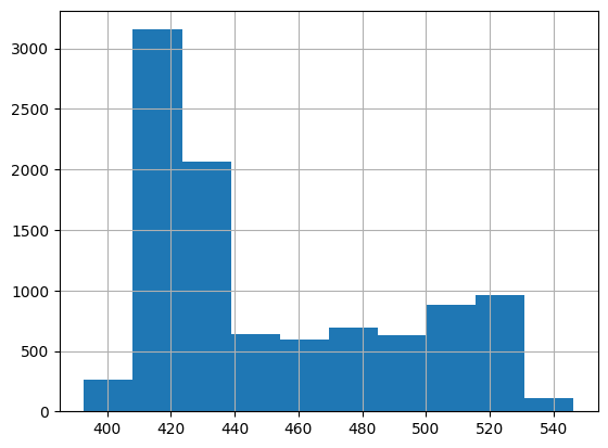
You can evaluate minimum detectable effect for your data. This will be the smallest true effect obtained from the changes, which the statistical criterion will be able to detect with confidence
[43]:
mde = experiment.calc_mde(data=splitted_data, group_field="group", target_field=mde_target)
mde
[43]:
(0.88, 0.02)
You can also calculate the amount of data you need to have in order to determine the minimum effect of the test.
[44]:
experiment.calc_sample_size(data=splitted_data, target_field=mde_target, mde=5)
[44]:
1949.4372012485414
Chi2 Test
[45]:
target = ['post_spends', 'pre_spends']
treated_field = 'treat'
[46]:
experiment = AATest(target_fields=target)
[47]:
experiment.calc_chi2(data, treated_field)
[47]:
{'post_spends': 4.2708618195357307e-129, 'pre_spends': 0.3904626181767134}